Create a Smooth Vector Plot Layer

Usage

geom_vector_smooth(
  mapping = NULL,
  data = NULL,
  stat = "vector_smooth",
  position = "identity",
  ...,
  na.rm = FALSE,
  show.legend = NA,
  inherit.aes = TRUE,
  n = c(11, 11),
  method = "gam",
  se = TRUE,
  se.circle = FALSE,
  pi_type = "ellipse",
  conf_level = c(0.95, NA),
  formula = cbind(fx, fy) ~ x * y,
  eval_points = NULL,
  arrow = grid::arrow(angle = 20, length = unit(0.015, "npc"), type = "closed")
)

GeomVectorSmooth

Format

An object of class GeomVectorSmooth (inherits from GeomSegment, Geom, ggproto, gg) of length 6.

Arguments

mapping

A set of aesthetic mappings created by ggplot2::aes(). Required: Must include x and y; vector displacements are defined by fx and fy.

data

A data frame containing the raw vector data.

stat

The statistical transformation to use on the data (default: "vector_smooth").

position

Position adjustment, either as a string or the result of a position adjustment function.

...

Other arguments passed to ggplot2::layer() and the underlying geometry/stat.

n

An integer vector specifying the number of grid points along each axis for smoothing.

method

Character. Specifies the smoothing method. Supported options include "lm", "kriging", and "gam". The "lm" method fits a multivariate linear model, "kriging" uses a cokriging approach via the gstat package, and "gam" fits separate generalized additive models for fx and fy (with predictions assumed independent, i.e., zero covariance).

se

Logical. If TRUE, prediction (confidence) intervals are computed and plotted.

se.circle

Logical. Defaults to FALSE. If TRUE, circles are drawn around the origin of each vector. By default, the circle’s radius is computed as the magnitude of the predicted vector.

pi_type

Character. Determines the display style for prediction intervals:

• "wedge" (default): Angular wedges are drawn.

• "ellipse": Ellipses are used to represent the covariance of the predictions. If pi_type is set to "ellipse" and eval_points is NULL, it will revert to "wedge".

conf_level

Numeric. Specifies the confidence level for the prediction intervals. Default is 0.95.

formula

A formula specifying the multivariate linear model used for smoothing. The default is cbind(fx, fy) ~ x * y.

eval_points

A data frame of evaluation points. If provided, these specify the grid where the smoothing model is evaluated. If NULL, a grid is generated based on n.

arrow

A grid::arrow() specification for arrowheads on the smoothed vectors.

Value

A ggplot2 layer that can be added to a plot to create a smooth vector field visualization.

Details

geom_vector_smooth() creates a ggplot2 layer that visualizes a smooth vector field. It takes raw vector data and applies smoothing (via a multivariate linear model) to estimate the underlying vector field. This functionality is analogous to geom_smooth() in ggplot2 but is tailored for vector data rather than scalar responses.

Aesthetics

geom_vector_smooth() supports the following aesthetics (required aesthetics are in bold):

• x: The x-coordinate of the vector's starting point.

• y: The y-coordinate of the vector's starting point.

• fx: The horizontal component of the vector displacement.

• fy: The vertical component of the vector displacement.

• color: The color of the vector lines.

• linewidth: The thickness of the vector lines.

• linetype: The type of the vector lines (e.g., solid, dashed).

• alpha: The transparency level of the vectors.

• arrow: An aesthetic that can be used to modify arrowhead properties.

Details

Multivariate Linear Model: The "lm" method fits a multivariate linear model to predict vector displacements (fx and fy) based on the coordinates x and y, including interaction terms (x * y). This model smooths the raw vector data to provide an estimate of the underlying vector field.

Prediction Intervals: When se = TRUE, prediction intervals are computed for the smoothed vectors. Two types of intervals are supported:

• Ellipse: Ellipses represent the joint uncertainty (covariance) in the predicted fx and fy.

• Wedge: Wedges (angular sectors) indicate the range of possible vector directions and magnitudes. The type of interval displayed is controlled by pi_type, and the confidence level is set via conf_level.

Examples

# Function to generate vectors
generate_vectors <- function(v) {
  x <- v[1]
  y <- v[2]
  c(
    sin(x) + sin(y) + rnorm(1, 5, 1),
    sin(x) - sin(y) - rnorm(1, 5, 1)
  )
}

# Set seed for reproducibility
set.seed(123)

# Create sample points and compute vectors
sample_points <- data.frame(
  x = runif(30, 0, 10),
  y = runif(30, 0, 10)
)

result <- t(apply(sample_points, 1, generate_vectors))

sample_points$xend <- result[, 1]
sample_points$yend <- result[, 2]
sample_points$fx <- sample_points$xend - sample_points$x
sample_points$fy <- sample_points$yend - sample_points$y
sample_points$distance <- sqrt(sample_points$fx^2 + sample_points$fy^2)
sample_points$angle <- atan2(sample_points$fy, sample_points$fx)

# Define evaluation points
eval_points <- data.frame(
  x = c(0, 7.5),
  y = c(10, 5)
)

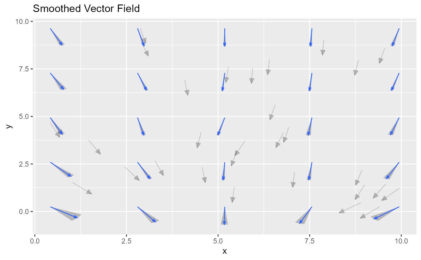
# Example 1:
ggplot(sample_points, aes(x = x, y = y)) +
  geom_vector(aes(fx = fx, fy = fy, color = NULL), center = FALSE, alpha = 0.2) +
  geom_vector_smooth(aes(fx = fx, fy = fy), n = 5) +
  ggtitle("Smoothed Vector Field")
#> Warning: ! eval_points is `NULL`; changing pi_type from "ellipse" to "wedge".


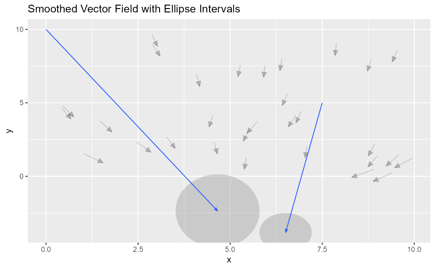
# Example 2: Ellipse with eval_points
ggplot(sample_points, aes(x = x, y = y)) +
  geom_vector(aes(fx = fx, fy = fy, color = NULL), center = FALSE, alpha = 0.2) +
  geom_vector_smooth(aes(fx = fx, fy = fy), eval_points = eval_points, conf_level = c(0.9)) +
  ggtitle("Smoothed Vector Field with Ellipse Intervals")


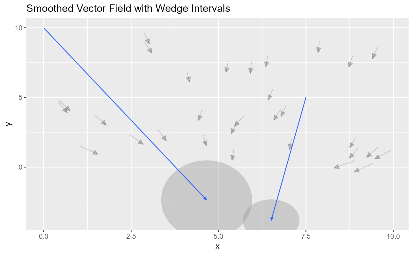
# Example 3: Wedge with eval_points
ggplot(sample_points, aes(x = x, y = y)) +
  geom_vector(aes(fx = fx, fy = fy, color = NULL), center = FALSE, alpha = 0.2) +
  geom_vector_smooth(aes(fx = fx, fy = fy), eval_points = eval_points, pi_type = "ellipse") +
  ggtitle("Smoothed Vector Field with Wedge Intervals")