
This post serves two purposes: it’s both an analysis of the Lucky $even game on The Price Is Right and a tutorial on data analysis in R – covering web scraping, data wrangling, visualization, and simulation. All code is folded by default; click “Show code” to expand any block and follow along.
In previous posts, I’ve looked at spinning the big wheel and winning Pay the Rent on The Price Is Right. This time, let’s tackle Lucky $even – a deceptively simple game where a little number sense goes a long way.
How Lucky $even Works #
The contestant plays for a car with a 5-digit price (e.g., $25,475). The first digit is revealed for free. The contestant starts with $7 and must guess the remaining four digits one at a time.
After each guess, the contestant loses money equal to how far off they were:
$$\text{cost} = |\text{guess} - \text{actual}|$$
If they guess exactly right, they lose nothing. After all four guesses, the contestant wins if:
$$M_{\text{remaining}} = 7 - \sum_{i=1}^{4} |\text{guess}_i - \text{actual}_i| \geq 1$$
The question is: what should you guess for each digit to maximize your chance of winning?
What We’ll Do #
- Scrape game-by-game results from the Price Is Right Wiki
- Reconstruct actual car price digits from the money trail
- Examine digit distributions by position (thousands, hundreds, tens, ones)
- Find the optimal guess for each position
- Simulate win rates under different strategies
Scrape & Clean the Data #
The Price Is Right Wiki has gallery pages documenting every playing of Lucky $even. Each image caption describes a digit guess: “says 5 and is exactly right”, “says 4 and has $3 left”, or “says 6 and has lost all of her money.” We scrape the 2010s and 2020s pages (~168 games), parse the captions with regex, and track money through each game.
library(tidyverse)
library(lubridate)
library(rvest)
library(scales)
scrape_page <- function(url) {
page <- read_html(url)
content <- page |> html_element(".mw-parser-output")
nodes <- content |> html_elements(".mw-headline, .lightbox-caption")
tibble(
text = nodes |> html_text2(),
type = if_else(str_detect(nodes |> html_attr("class"), "mw-headline"), "heading", "caption")
)
}
raw_data <- map_dfr(
c("https://priceisright.fandom.com/wiki/Lucky_%24even/Gallery/2010s",
"https://priceisright.fandom.com/wiki/Lucky_%24even/Gallery/2020s"),
scrape_page, .id = "page"
)
# Group captions under their game heading, parse guess details
games_raw <- raw_data |>
mutate(game_id = cumsum(type == "heading")) |>
filter(game_id > 0)
captions <- games_raw |>
filter(type == "caption", str_detect(text, "says \\d")) |>
mutate(
guess = as.integer(str_extract(text, "says (\\d)", group = 1)),
exactly_right = str_detect(text, "exactly right"),
money_left = as.integer(str_extract(text, "\\$(\\d+) left", group = 1)),
lost_all = str_detect(text, "lost all|lost .* only dollar")
)With the captions parsed, we track money through each game. The contestant starts with $7 (with rare $8 or $10 exceptions we’ll exclude). For each digit (i), the money updates as:
$$M_i = M_{i-1} - |\text{guess}_i - \text{actual}_i|$$
where (M_0 = 7). The contestant wins if (M_4 \geq 1).
# Detect non-standard starting money and exclude those games
starting_money_overrides <- games_raw |>
  filter(type == "caption") |>
  mutate(
    is_lucky_eight = str_detect(text, regex("Lucky Eight|\\$8 instead", ignore_case = TRUE)),
    is_lucky_ten = str_detect(text, regex("Lucky Ten|\\$10 instead", ignore_case = TRUE))
  ) |>
  group_by(game_id) |>
  summarize(starting_money = case_when(
    any(is_lucky_ten) ~ 10L, any(is_lucky_eight) ~ 8L, TRUE ~ 7L
  ))

compute_money_trail <- function(df, start_money) {
  n <- nrow(df)
  mb <- ma <- integer(n)
  for (i in seq_len(n)) {
    mb[i] <- if (i == 1) start_money else ma[i - 1]
    ma[i] <- case_when(
      df$exactly_right[i] ~ mb[i], df$lost_all[i] ~ 0L,
      !is.na(df$money_left[i]) ~ df$money_left[i], TRUE ~ NA_integer_
    )
  }
  df |> mutate(money_before = mb, money_after = ma)
}

game_data <- captions |>
  group_by(game_id) |> mutate(digit_position = row_number()) |> ungroup() |>
  left_join(starting_money_overrides, by = "game_id") |>
  group_by(game_id) |>
  group_modify(~ compute_money_trail(.x, .x$starting_money[1])) |>
  ungroup() |>
  mutate(cost = money_before - money_after)

# Reconstruct actual digits: actual = guess ± cost (pick whichever falls in 0-9)
game_data <- game_data |>
  mutate(
    option_high = guess + cost, option_low = guess - cost,
    actual = case_when(
      cost == 0 ~ guess,
      option_high > 9 & option_low >= 0 ~ option_low,
      option_low < 0 & option_high <= 9 ~ option_high,
      option_high <= 9 & option_low >= 0 ~ NA_integer_,
      TRUE ~ NA_integer_
    ),
    ambiguous = cost > 0 & option_high <= 9 & option_low >= 0
  )

# Keep standard $7 games with all 4 guesses
standard_games <- game_data |>
  filter(starting_money == 7) |>
  group_by(game_id) |> filter(max(digit_position) == 4) |> ungroup()

game_outcomes <- standard_games |>
  group_by(game_id) |>
  summarize(final_money = last(money_after), won = final_money >= 1, .groups = "drop")

cat("Games:", nrow(game_outcomes), "| Wins:", sum(game_outcomes$won, na.rm = TRUE),
    "(", percent(mean(game_outcomes$won, na.rm = TRUE)), ") |",
    "Unambiguous digits:", sum(!is.na(standard_games$actual)), "/", nrow(standard_games), "\n")
## Games: 109 | Wins: 57 ( 53% ) | Unambiguous digits: 149 / 436Digit Distributions by Position #
One wrinkle: the wiki captions tell us the cost of each guess (how much money the contestant lost), but not always the actual digit. Since (\text{cost} = |\text{guess} - \text{actual}|), there are sometimes two solutions:
$$\text{actual} = \text{guess} + \text{cost} \quad \text{or} \quad \text{actual} = \text{guess} - \text{cost}$$
For example, if a contestant guesses 5 and loses $2, the actual digit was either (5 - 2 = 3) or (5 + 2 = 7) – we can’t tell which. That’s an ambiguous case. But if a contestant guesses 8 and loses $3, the actual could be (8 - 3 = 5) or (8 + 3 = 11). Since 11 isn’t a valid digit (must be 0-9), the actual must be 5 – that’s unambiguous.
The four digits correspond to the thousands, hundreds, tens, and ones place of the car price. Let’s start by looking at the distribution of actual digits for each position, using only the unambiguous cases.
position_labels <- c("1" = "Thousands", "2" = "Hundreds", "3" = "Tens", "4" = "Ones")

digit_dist <- standard_games |>
  filter(!is.na(actual)) |>
  mutate(position_label = factor(position_labels[as.character(digit_position)],
                                  levels = c("Thousands", "Hundreds", "Tens", "Ones")))

ggplot(digit_dist, aes(x = factor(actual))) +
  geom_bar(fill = "steelblue", alpha = 0.8) +
  facet_wrap(~ position_label, scales = "free_y") +
  labs(
    title = "Distribution of Actual Digits in Lucky $even",
    subtitle = "Based on unambiguous cases from ~168 games (2010s-2020s)",
    x = "Digit Value",
    y = "Count"
  ) +
  theme_minimal(base_size = 14)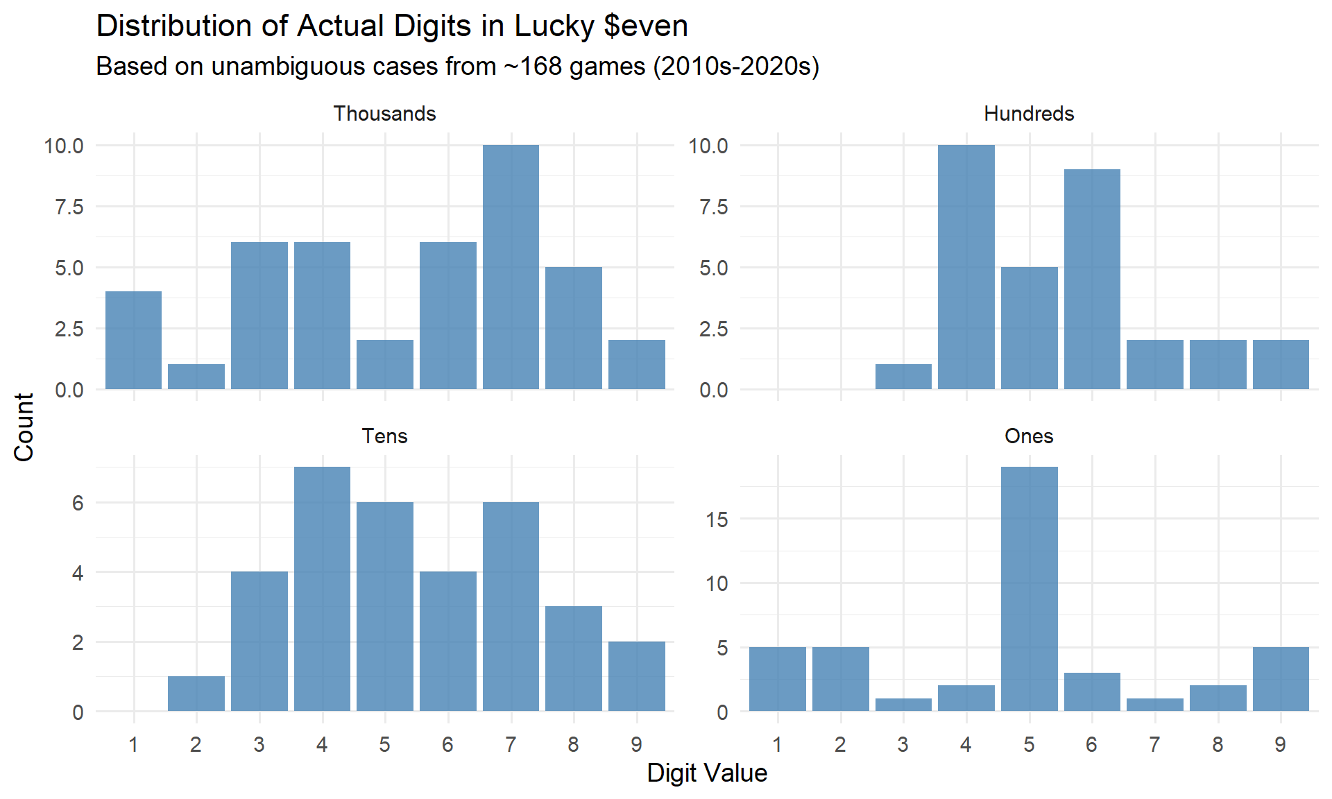
For the ambiguous cases, we can include both possibilities weighted at 0.5 each to get a fuller picture:
# Build weighted digit distribution including ambiguous cases
weighted_dist <- bind_rows(
  # Unambiguous cases: weight = 1
  standard_games |>
    filter(!is.na(actual)) |>
    transmute(digit_position, actual, weight = 1),
  # Ambiguous cases: both options weighted at 0.5
  standard_games |>
    filter(ambiguous) |>
    transmute(digit_position, actual = option_high, weight = 0.5),
  standard_games |>
    filter(ambiguous) |>
    transmute(digit_position, actual = option_low, weight = 0.5)
) |>
  mutate(position_label = factor(position_labels[as.character(digit_position)],
                                  levels = c("Thousands", "Hundreds", "Tens", "Ones")))

ggplot(weighted_dist, aes(x = factor(actual), weight = weight)) +
  geom_bar(fill = "darkgreen", alpha = 0.8) +
  facet_wrap(~ position_label, scales = "free_y") +
  labs(
    title = "Weighted Digit Distribution (Including Ambiguous Cases)",
    subtitle = "Ambiguous cases contribute 0.5 to each possible digit",
    x = "Digit Value",
    y = "Weighted Count"
  ) +
  theme_minimal(base_size = 14)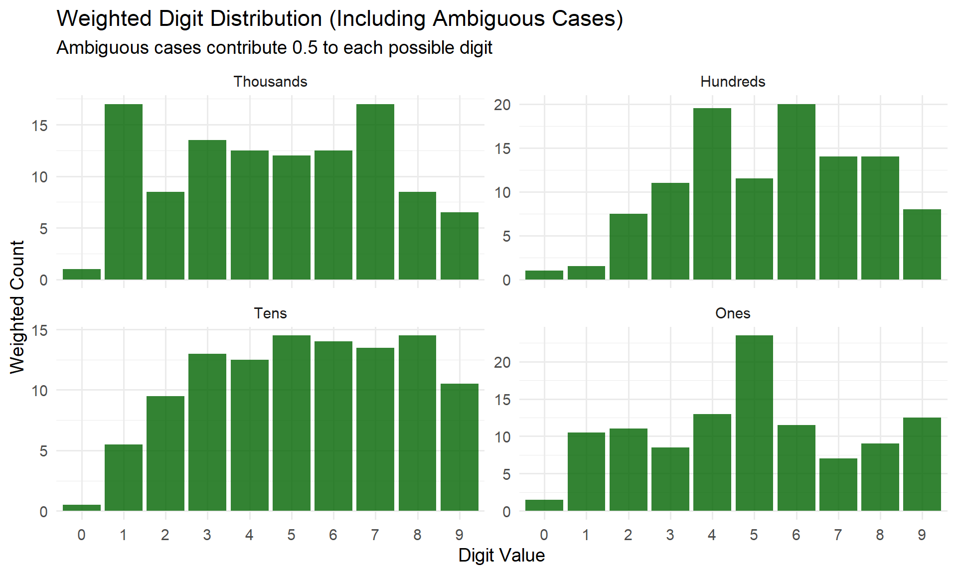
Optimal Strategy #
For each digit position, we want to choose the guess (g) that minimizes the expected cost:
$$g^* = \arg\min_{g \in {0,\ldots,9}} ; \mathbb{E}\left[|g - D|\right] = \arg\min_{g} \sum_{d=0}^{9} |g - d| \cdot P(D = d)$$
where (D) is the random variable for the actual digit at that position. This is minimized by choosing the weighted median of the digit distribution.
Let’s compute the expected cost of every possible guess (0-9) at each position:
# Compute expected cost for each guess at each position
expected_costs <- weighted_dist |>
  group_by(digit_position, actual) |>
  summarize(prob_weight = sum(weight), .groups = "drop") |>
  group_by(digit_position) |>
  mutate(prob = prob_weight / sum(prob_weight)) |>
  ungroup() |>
  crossing(guess_candidate = 0:9) |>
  mutate(cost = abs(guess_candidate - actual) * prob) |>
  group_by(digit_position, guess_candidate) |>
  summarize(expected_cost = sum(cost), .groups = "drop") |>
  mutate(position_label = factor(position_labels[as.character(digit_position)],
                                  levels = c("Thousands", "Hundreds", "Tens", "Ones")))

# Find optimal guess per position
optimal <- expected_costs |>
  group_by(digit_position, position_label) |>
  slice_min(expected_cost, n = 1, with_ties = FALSE) |>
  ungroup()

ggplot(expected_costs, aes(x = guess_candidate, y = expected_cost)) +
  geom_line(color = "steelblue", linewidth = 1) +
  geom_point(data = optimal, aes(x = guess_candidate, y = expected_cost),
             color = "red", size = 4) +
  geom_text(data = optimal, aes(x = guess_candidate, y = expected_cost,
                                 label = paste0("Guess ", guess_candidate)),
            vjust = -1.2, color = "red", fontface = "bold") +
  facet_wrap(~ position_label) +
  scale_x_continuous(breaks = 0:9) +
  labs(
    title = "Expected Cost by Guess Value at Each Position",
    subtitle = "Red dot = optimal guess (minimizes expected dollar loss)",
    x = "Guess",
    y = "Expected Cost ($)"
  ) +
  theme_minimal(base_size = 14)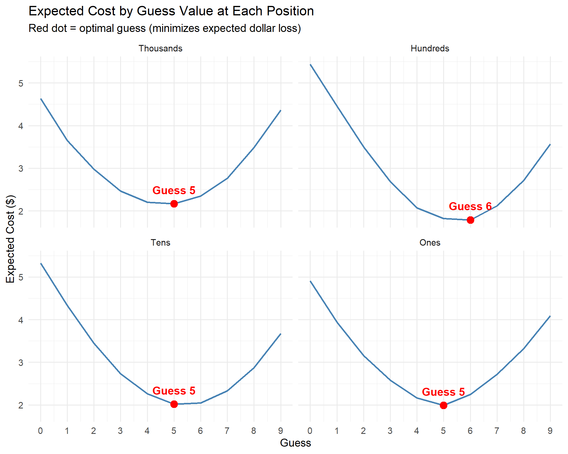
# Summary table
optimal |>
  select(Position = position_label, `Optimal Guess` = guess_candidate,
         `Expected Cost` = expected_cost) |>
  mutate(`Expected Cost` = round(`Expected Cost`, 2)) |>
knitr::kable()| Position | Optimal Guess | Expected Cost |
|---|---|---|
| Thousands | 5 | 2.17 |
| Hundreds | 6 | 1.79 |
| Tens | 5 | 2.02 |
| Ones | 5 | 1.99 |
The total expected cost across all four guesses using the optimal strategy is the sum across positions:
$$\text{Total Expected Cost} = \sum_{i=1}^{4} \mathbb{E}\left[|g^*_i - D_i|\right]$$
total_optimal_cost <- sum(optimal$expected_cost)
cat("Total expected cost: $", round(total_optimal_cost, 2), "\n")
## Total expected cost: $ 7.96cat("Expected money remaining: $", round(7 - total_optimal_cost, 2), "\n")## Expected money remaining: $ -0.96Simulation: Comparing Strategies #
Let’s put this to the test. We’ll simulate 100,000 games under four strategies and compare win rates. In each simulated game, we draw digits from the empirical distributions and check whether the contestant wins:
$$P(\text{win} \mid \text{strategy}) = P\left(7 - \sum_{i=1}^{4} |g_i - D_i| \geq 1\right)$$
The four strategies:
- Optimal – guess the cost-minimizing digit (g^*_i) at each position
- Always 5 – guess (g_i = 5) for every digit (the “middle of the road” approach)
- Always Mode – guess the most common digit at each position
- Random – guess a random digit each time
# Build digit probability distributions per position
digit_probs <- weighted_dist |>
  group_by(digit_position, actual) |>
  summarize(w = sum(weight), .groups = "drop") |>
  group_by(digit_position) |>
  mutate(prob = w / sum(w)) |>
  ungroup()

# Ensure all digits 0-9 represented for each position
full_probs <- crossing(digit_position = 1:4, actual = 0:9) |>
  left_join(digit_probs |> select(digit_position, actual, prob),
            by = c("digit_position", "actual")) |>
  replace_na(list(prob = 0)) |>
  group_by(digit_position) |>
  mutate(prob = prob / sum(prob)) |>  # renormalize
  ungroup()

prob_matrix <- full_probs |>
  pivot_wider(names_from = actual, values_from = prob, names_prefix = "d") |>
  select(-digit_position) |>
  as.matrix()

# Mode per position
mode_guesses <- full_probs |>
  group_by(digit_position) |>
  slice_max(prob, n = 1, with_ties = FALSE) |>
  pull(actual)

optimal_guesses <- optimal$guess_candidate

# Simulation function
simulate_strategy <- function(strategy_fn, n_games = 100000) {
  results <- replicate(n_games, {
    money <- 7
    for (pos in 1:4) {
      actual_digit <- sample(0:9, 1, prob = prob_matrix[pos, ])
      guess <- strategy_fn(pos)
      money <- money - abs(guess - actual_digit)
      if (money <= 0) break
    }
    money
  })
  results
}

set.seed(42)
results <- tibble(
  strategy = c("Optimal", "Always 5", "Always Mode", "Random"),
  money = list(
    simulate_strategy(function(pos) optimal_guesses[pos]),
    simulate_strategy(function(pos) 5),
    simulate_strategy(function(pos) mode_guesses[pos]),
    simulate_strategy(function(pos) sample(0:9, 1))
  )
) |>
  unnest(money) |>
  mutate(won = money >= 1)
# Win rate comparison
win_rates <- results |>
group_by(strategy) |>
summarize(
win_rate = mean(won),
avg_money = mean(money),
.groups = "drop"
) |>
mutate(strategy = fct_reorder(strategy, win_rate))
ggplot(win_rates, aes(x = strategy, y = win_rate, fill = strategy)) +
geom_col(alpha = 0.8, show.legend = FALSE) +
geom_text(aes(label = percent(win_rate, accuracy = 0.1)), vjust = -0.5, fontface = "bold") +
scale_y_continuous(labels = percent, limits = c(0, 1)) +
scale_fill_brewer(palette = "Set2") +
labs(
title = "Win Rate by Strategy (100,000 Simulated Games)",
x = "Strategy",
y = "Win Rate"
) +
theme_minimal(base_size = 14)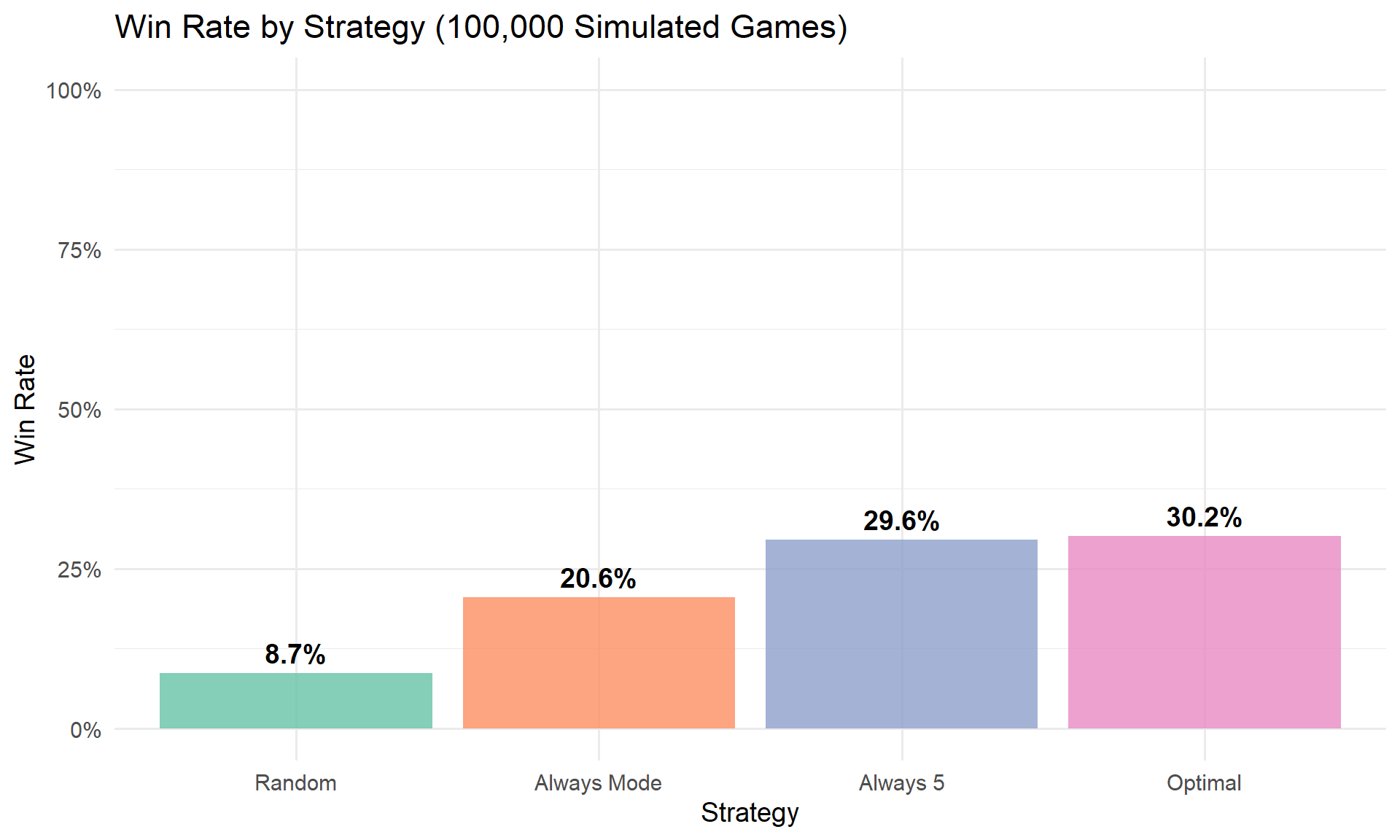
# Distribution of remaining money
ggplot(results |> filter(strategy %in% c("Optimal", "Always 5")),
       aes(x = money, fill = strategy)) +
  geom_histogram(binwidth = 1, position = "dodge", alpha = 0.7) +
  annotate("rect", xmin = 1, xmax = Inf, ymin = -Inf, ymax = Inf,
           fill = "green", alpha = 0.08) +
  annotate("text", x = 4, y = Inf, label = "Win (\u2265 $1)",
           vjust = 2, color = "darkgreen", fontface = "bold", size = 5) +
  labs(
    title = "Distribution of Remaining Money",
    subtitle = "Optimal vs. Always-5 Strategy",
    x = "Money Remaining ($)",
    y = "Count",
    fill = "Strategy"
  ) +
  scale_x_continuous(breaks = scales::breaks_width(1)) +
  theme_minimal(base_size = 14)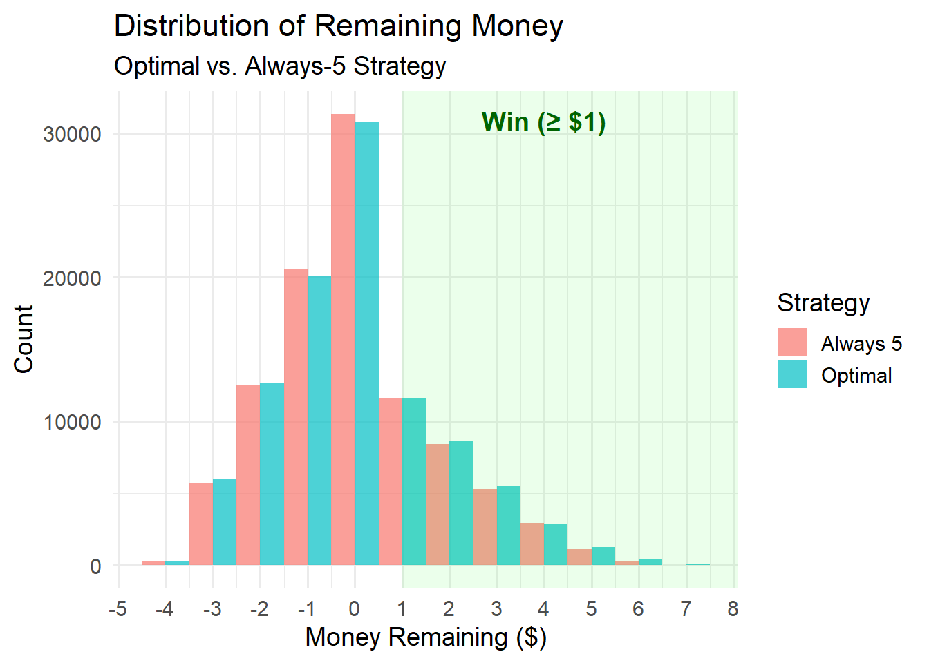
win_rates |>
  mutate(
    win_rate = percent(win_rate, accuracy = 0.1),
    avg_money = paste0("$", round(avg_money, 2))
  ) |>
  arrange(desc(win_rate)) |>
  rename(Strategy = strategy, `Win Rate` = win_rate, `Avg Money Remaining` = avg_money) |>
knitr::kable()| Strategy | Win Rate | Avg Money Remaining |
|---|---|---|
| Random | 8.7% | $-1.41 |
| Optimal | 30.2% | $0.01 |
| Always 5 | 29.6% | $-0.01 |
| Always Mode | 20.6% | $-0.24 |
How Does This Compare to Reality? #
actual_win_rate <- mean(game_outcomes$won, na.rm = TRUE)
cat("Actual win rate from wiki data:", percent(actual_win_rate, accuracy = 0.1), "\n")
## Actual win rate from wiki data: 52.8%cat("Optimal strategy win rate:", percent(win_rates$win_rate[win_rates$strategy == "Optimal"]), "\n")## Optimal strategy win rate: 30%Contestants on the show don’t play optimally – they’re guessing under pressure without data. But the actual win rate gives us a nice benchmark. The gap between reality and optimal represents how much better contestants could do with a data-driven approach.
Conclusion #
Lucky $even rewards contestants who have good intuition about car prices. But even without knowing the exact price, a data-driven strategy can meaningfully improve your odds:
- Car price digits are not uniformly distributed. Certain digits appear far more often at each position, driven by how manufacturers price their cars.
- The “optimal” strategy is essentially just guessing 5 every time. The data-driven median produces mostly 5s with one position suggesting a 6 – but with only ~168 games of data, that difference is likely noise. The takeaway isn’t a magic sequence of digits; it’s that 5 is a remarkably good default guess because car price digits tend to cluster in the middle of the 0-9 range.
- Guessing 5 every time already does quite well compared to random guessing or other naive strategies. You don’t need to memorize anything fancy – just guess 5 and hope for the best.
So the next time Drew Carey calls you down and you find yourself playing Lucky $even, the strategy is simple: guess 5 for every digit. It won’t guarantee a win, but the data says it gives you the best shot. Just don’t forget to bring that last dollar.