# A tibble: 6 × 10
  Education       Sex   Occupation   Age Earnings MaritalStatus Race  FamilySize
  <chr>           <chr> <chr>      <dbl>    <dbl> <chr>         <chr>      <dbl>
1 Bachelors       M     40: Offic…    49   220000 Married       White          5
2 Some College/A… F     53: Never…    51        0 Married       White          5
3 Less than HS    F     39: Retai…    20     8000 Never Married White          5
4 Less than HS    M     8: Comput…    16     4000 Never Married White          5
5 Less than HS    F     53: Never…    80        0 Widowed       White          5
6 Less than HS    M     32: Chefs…    27    17350 Never Married Black          2
# ℹ 2 more variables: FamilyMakeup <chr>, Age_squared <dbl>MA206 Tidyverse Lab
Save This File
Save this .Rmd file with the title Lastname_Firstname_Tidyverse-Lab.Rmd into your RStudio folder.
Importing Libraries
The Research Question
Type your research question here.
Summary of the ________ Data Set
Insert your data set name above and type your summary here. You will fill out the table shortly.
The Data Set
Name and load your data set below.
The output of the above code, in conjunction with any provided data dictionary, should enable you to complete the table below. Remove the information from the wage data set and use your own.
| Variable | Column Name | Units | Variable Type |
|---|---|---|---|
| Education | Education | N/A | Categorical |
| Sex | Sex | N/A | Categorical |
| Occupation | Occupation | N/A | Categorical |
| Age | Age | Years | Quantitative |
| Earnings | Earnings | Dollars | Quantitative |
| Marital Status | MaritalStatus | N/A | Categorical |
| Race | Race | N/A | Categorical |
| Family Size | FamilySize | N/A | Categorical |
| Family Makeup | FamilyMakeup | N/A | Categorical |
| Age Squared | Age_squared | Years | Quantitative |
Practice
Use the below space to practice calling, selecting, filtering, summarizing, grouping by, and mutating variables.
[1] 49 51 20 16 80 27# A tibble: 180,084 × 2
Age Earnings
<dbl> <dbl>
1 49 220000
2 51 0
3 20 8000
4 16 4000
5 80 0
6 27 17350
7 24 12000
8 62 25480
9 70 0
10 53 6000
# ℹ 180,074 more rows# A tibble: 37,174 × 10
Education Sex Occupation Age Earnings MaritalStatus Race FamilySize
<chr> <chr> <chr> <dbl> <dbl> <chr> <chr> <dbl>
1 Bachelors M 40: Office … 49 220000 Married White 5
2 Bachelors M 31: Animal … 62 25480 Never Married White 1
3 Bachelors M 8: Computer… 52 70200 Married Asian 6
4 Less than HS M 53: Never W… 50 0 Married White 3
5 Less than HS M 53: Never W… 62 0 Married White 2
6 Less than HS M 51: Transpo… 55 40000 Never Married White 1
7 Less than HS M 49: Product… 51 83000 Married White 3
8 Less than HS M 40: Office … 47 35000 Married White 4
9 Less than HS M 38: Retail … 70 0 Married White 2
10 Less than HS M 3: Educatio… 62 0 Divorced White 1
# ℹ 37,164 more rows
# ℹ 2 more variables: FamilyMakeup <chr>, Age_squared <dbl># A tibble: 1 × 1
avg
<dbl>
1 37.0# A tibble: 2 × 2
Sex ave
<chr> <dbl>
1 F 37.9
2 M 36.0# A tibble: 180,084 × 1
weird_age
<dbl>
1 98
2 102
3 40
4 32
5 160
6 54
7 48
8 124
9 140
10 106
# ℹ 180,074 more rowsExplore Your Variables
Response Variable
Type the name, description, and units of your response variable here. Remember that this is a quantitative variable.
   Min. 1st Qu.  Median    Mean 3rd Qu.    Max.
0 0 0 24813 35000 1609999 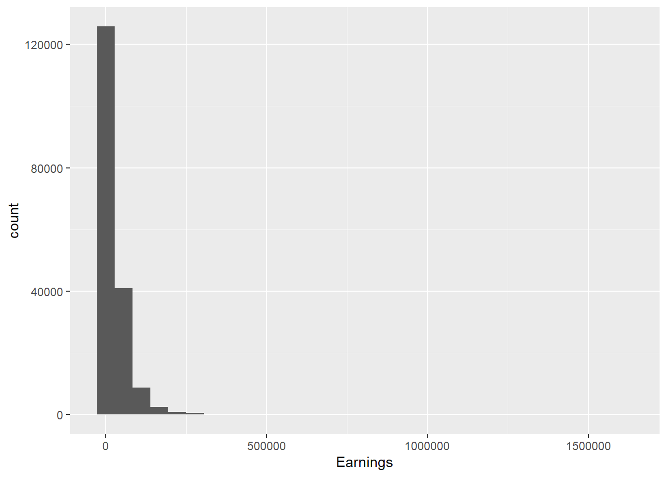
In 1-2 sentences, describe this variable’s data. Which visualization is better, and why? Are there any questions that you have after exploring? Add code chunks below if you’d like to do some more exploration.
Quantitative Explantory Variable #1
Type the name, description, and units of your quantitative variable here.
# A tibble: 1 × 3
    mean      s      n
   <dbl>  <dbl>  <int>
1 24813. 54264. 180084
In 1-2 sentences, describe this variable’s data. Which visualization is better, and why? Are there any questions that you have after exploring? Add code chunks below if you’d like to do some more exploration.
Quantitative Explantory Variable #2
Type the name, description, and units of your quantitative variable here.
In 1-2 sentences, describe this variable’s data. Which visualization is better, and why? Are there any questions that you have after exploring? Add code chunks below if you’d like to do some more exploration.
Categorical Explanatory Variable #1
Type the name, description, and units of your categorical variable here. Remember that this will require different code than your quantitative variables.
    F     M
92693 87391 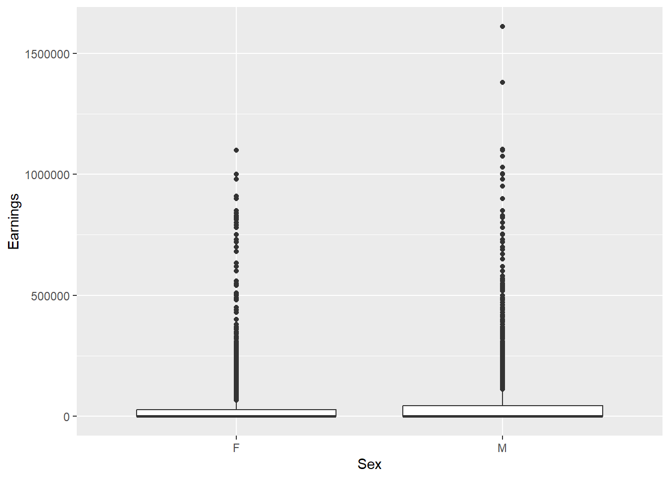
In 1-2 sentences, describe this variable’s data. Which visualization is better, and why? Are there any questions that you have after exploring? Add code chunks below if you’d like to do some more exploration.
Categorical Explanatory Variable #2
Type the name, description, and units of your categorical variable here. Remember that this will require different code than your quantitative variables.
In 1-2 sentences, describe this variable’s data. Which visualization is better, and why? Are there any questions that you have after exploring? Add code chunks below if you’d like to do some more exploration.
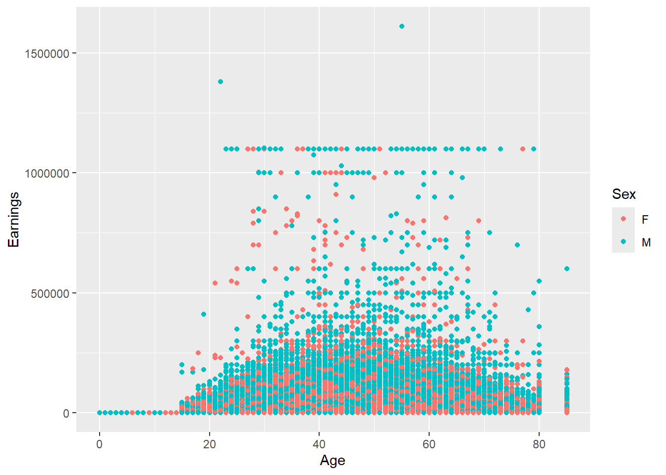
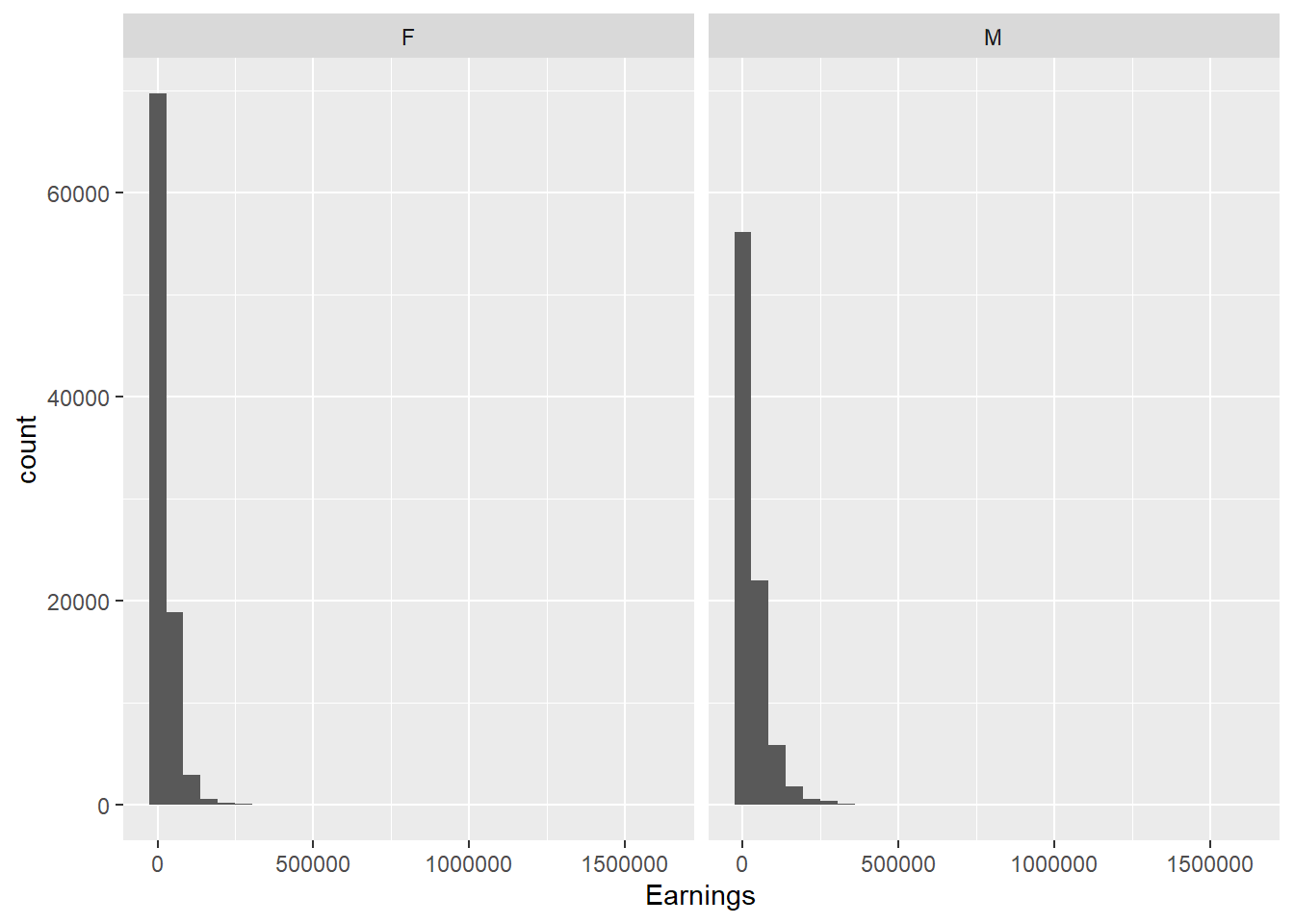
How are the variables associated?
Using ggplot, create visualizations that show relationships between your variables below. Since you have five variables, you will need at minimum four plots so that each variable is visualized at least once. It is possible to display relationships between 3+ variables in one plot; at least one of your plots should demonstrate mastery of this skill. Create more code chunks as needed.
Finish the tutorial
Test your skills by working through the code after the ggplot section of the Tutorial. These examples will help you gain a basic understanding of what is happening with specific commands or data structures within R, which will be useful to you over the course of the semester. Create more code chunks as needed.
Getting Ready to Submit!
Now that you’re done, you need to save this file (if the title is red, it has unsaved changes). RStudio does NOT autosave while you work, so CTRL+S early and often. Next, press the Knit button up top with the yarn icon. This will create an HTML file, because that was specified in the header. Save your HTML file with the name Lastname_Firstname_Tidyverse-Lab.html. Then, open the HTML file and print, using the `Microsoft Print to PDF" option to save asLastname_Firstname_Tidyverse-Lab.pdf`. This PDF file is what you will submit on Canvas for Milestone 2.