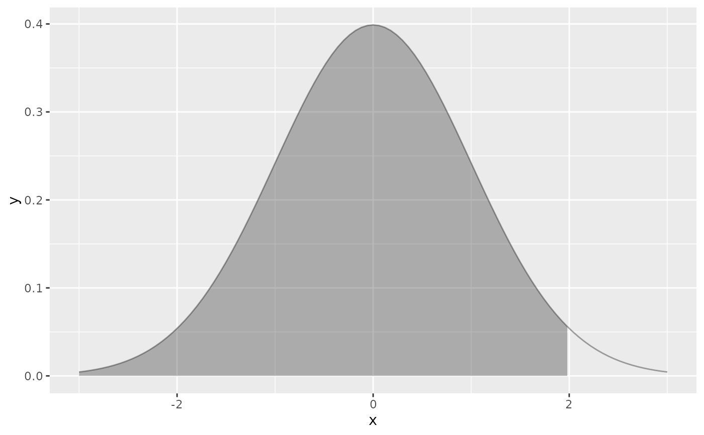
geom_pdf() computes a probability density function and plots it as a filled area.
This function is similar to ggplot2::geom_function(), but it shades the area corresponding to
a given proportion of the total density.
Usage
geom_pdf(
  mapping = NULL,
  data = NULL,
  stat = StatPDF,
  position = "identity",
  ...,
  na.rm = FALSE,
  show.legend = NA,
  inherit.aes = FALSE,
  fun = NULL,
  cdf_fun = NULL,
  survival_fun = NULL,
  qf_fun = NULL,
  xlim = NULL,
  n = 101,
  args = list(),
  fill = "grey20",
  color = "black",
  linewidth = NULL,
  alpha = 0.35,
  p = NULL,
  lower.tail = TRUE,
  p_lower = NULL,
  p_upper = NULL,
  shade_outside = FALSE,
  shade_hdr = NULL
)

StatPDF

GeomPDF
Format
An object of class StatPDF (inherits from Stat, ggproto, gg) of length 3.
An object of class GeomPDF (inherits from GeomArea, GeomRibbon, Geom, ggproto, gg) of length 2.
Arguments
- mapping
Set of aesthetic mappings created by
aes(). If specified andinherit.aes = TRUE(the default), it is combined with the default mapping at the top level of the plot. You must supplymappingif there is no plot mapping.- data
Ignored by
stat_function(), do not use.- stat
The statistical transformation to use on the data for this layer. When using a
geom_*()function to construct a layer, thestatargument can be used to override the default coupling between geoms and stats. Thestatargument accepts the following:A
Statggproto subclass, for exampleStatCount.A string naming the stat. To give the stat as a string, strip the function name of the
stat_prefix. For example, to usestat_count(), give the stat as"count".For more information and other ways to specify the stat, see the layer stat documentation.
- position
A position adjustment to use on the data for this layer. This can be used in various ways, including to prevent overplotting and improving the display. The
positionargument accepts the following:The result of calling a position function, such as
position_jitter(). This method allows for passing extra arguments to the position.A string naming the position adjustment. To give the position as a string, strip the function name of the
position_prefix. For example, to useposition_jitter(), give the position as"jitter".For more information and other ways to specify the position, see the layer position documentation.
- ...
Other arguments passed on to
layer()'sparamsargument. These arguments broadly fall into one of 4 categories below. Notably, further arguments to thepositionargument, or aesthetics that are required can not be passed through.... Unknown arguments that are not part of the 4 categories below are ignored.Static aesthetics that are not mapped to a scale, but are at a fixed value and apply to the layer as a whole. For example,
colour = "red"orlinewidth = 3. The geom's documentation has an Aesthetics section that lists the available options. The 'required' aesthetics cannot be passed on to theparams. Please note that while passing unmapped aesthetics as vectors is technically possible, the order and required length is not guaranteed to be parallel to the input data.When constructing a layer using a
stat_*()function, the...argument can be used to pass on parameters to thegeompart of the layer. An example of this isstat_density(geom = "area", outline.type = "both"). The geom's documentation lists which parameters it can accept.Inversely, when constructing a layer using a
geom_*()function, the...argument can be used to pass on parameters to thestatpart of the layer. An example of this isgeom_area(stat = "density", adjust = 0.5). The stat's documentation lists which parameters it can accept.The
key_glyphargument oflayer()may also be passed on through.... This can be one of the functions described as key glyphs, to change the display of the layer in the legend.
- na.rm
If
FALSE, the default, missing values are removed with a warning. IfTRUE, missing values are silently removed.- show.legend
Logical. Should this layer be included in the legends?
NA, the default, includes if any aesthetics are mapped.FALSEnever includes, andTRUEalways includes. It can also be a named logical vector to finely select the aesthetics to display. To include legend keys for all levels, even when no data exists, useTRUE. IfNA, all levels are shown in legend, but unobserved levels are omitted.- inherit.aes
If
FALSE, overrides the default aesthetics, rather than combining with them. This is most useful for helper functions that define both data and aesthetics and shouldn't inherit behaviour from the default plot specification, e.g.annotation_borders().- fun
A function to compute the density (e.g. dnorm). The function must accept a numeric vector as its first argument and return density values that integrate (approximately) to 1. Exactly one of
fun,cdf_fun,survival_fun, orqf_funmust be provided.- cdf_fun
A CDF function (e.g. pnorm). When supplied, the PDF is derived numerically via central finite differences. Exactly one of
fun,cdf_fun,survival_fun, orqf_funmust be provided.- survival_fun
A survival function (e.g.
function(x) 1 - pnorm(x)). When supplied, the CDF is computed as \(F(x) = 1 - S(x)\) and then differentiated to obtain the PDF. Exactly one offun,cdf_fun,survival_fun, orqf_funmust be provided.- qf_fun
A quantile function (e.g. qnorm). When supplied, the CDF is derived via interpolation and then differentiated to obtain the PDF. Exactly one of
fun,cdf_fun,survival_fun, orqf_funmust be provided.- xlim
A numeric vector of length 2 giving the x-range over which to evaluate the PDF.
- n
(defaults to 101)Number of points at which to evaluate
fun.- args
A named list of additional arguments to pass to
fun.- fill
Fill color for the shaded area.
- color
Line color for the outline of the density curve.
- linewidth
Line width for the outline of the density curve.
- alpha
Alpha transparency for the shaded area.
- p
(Optional) A numeric value between 0 and 1 specifying the cumulative probability threshold. The area will be shaded up until the point where the cumulative density reaches this value.
- lower.tail
Logical; if
TRUE(the default) the shaded area extends from the left end of the density up to the threshold. IfFALSE, the shading extends from the threshold to the right end.- p_lower
(Optional) A numeric value between 0 and 1 specifying the lower cumulative probability bound. Used with
p_upperfor two-sided shading.- p_upper
(Optional) A numeric value between 0 and 1 specifying the upper cumulative probability bound. Used with
p_lowerfor two-sided shading.- shade_outside
Logical; if
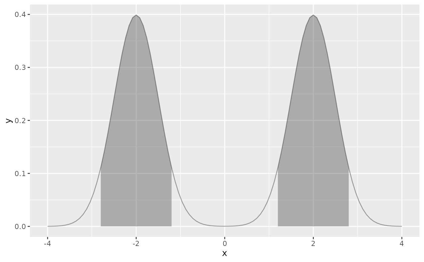
FALSE(the default) shading is applied betweenp_lowerandp_upper. IfTRUE, shading is applied to the tails outside that range.- shade_hdr
(Optional) A numeric value between 0 and 1 specifying the coverage of the highest density region (HDR) to shade. The HDR is the smallest region of the domain containing the specified probability mass; for multimodal densities it may be disconnected, producing multiple shaded intervals. Computed following the approach of doi:10.32614/RJ-2023-048 : density values are evaluated on the grid, normalized to sum to 1, sorted in descending order, and cumulated until the target coverage is reached; the density at that threshold determines which regions are shaded. Takes precedence over
p,p_lower, andp_upperif specified.