Introduction to ggfunction

Overview

ggfunction extends ggplot2 to visualize mathematical functions directly. It provides a unified interface organized around two families:

1. Dimensional taxonomy – functions classified by input/output dimension:
   • geom_function_1d_1d(): $\mathbb{R} \to \mathbb{R}$ (scalar to scalar)
   • geom_function_1d_2d(): $\mathbb{R} \to \mathbb{R}^2$ (parametric curves)
   • geom_function_2d_1d(): $\mathbb{R}^2 \to \mathbb{R}$ (scalar fields, raster/contour)
   • geom_function_2d_2d(): $\mathbb{R}^2 \to \mathbb{R}^2$ (vector fields)
2. Probability distributions – specialized geoms for distribution functions:
   • geom_pdf(): probability density function
   • geom_cdf(): cumulative distribution function
   • geom_pmf(): probability mass function (lollipop)
   • geom_qf(): quantile function
   • geom_cdf_discrete(): discrete CDF (right-continuous step function)
   • geom_qf_discrete(): discrete quantile function (left-continuous step function)
   • geom_survival_discrete(): discrete survival function $S(x) = 1 - F(x)$ (right-continuous step function)
   • geom_survival(): survival function $S(x) = 1 - F(x)$
   • geom_hf(): hazard function $h(x) = f(x)/S(x)$

Dimensional Taxonomy

1D to 1D: Scalar Functions

Plot any $f: \mathbb{R} \to \mathbb{R}$ with optional interval shading:

ggplot() +
  geom_function_1d_1d(fun = sin, xlim = c(0, 2 * pi))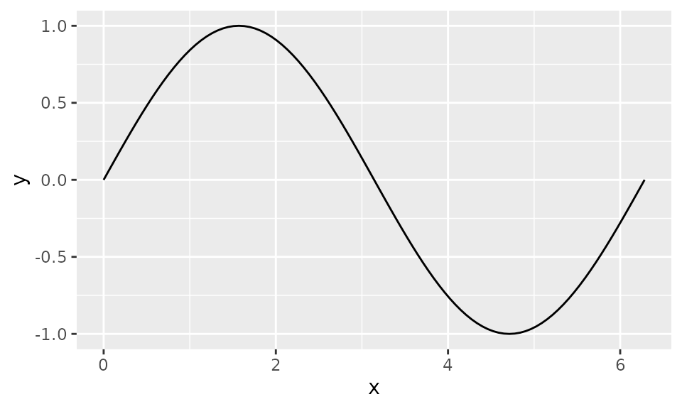

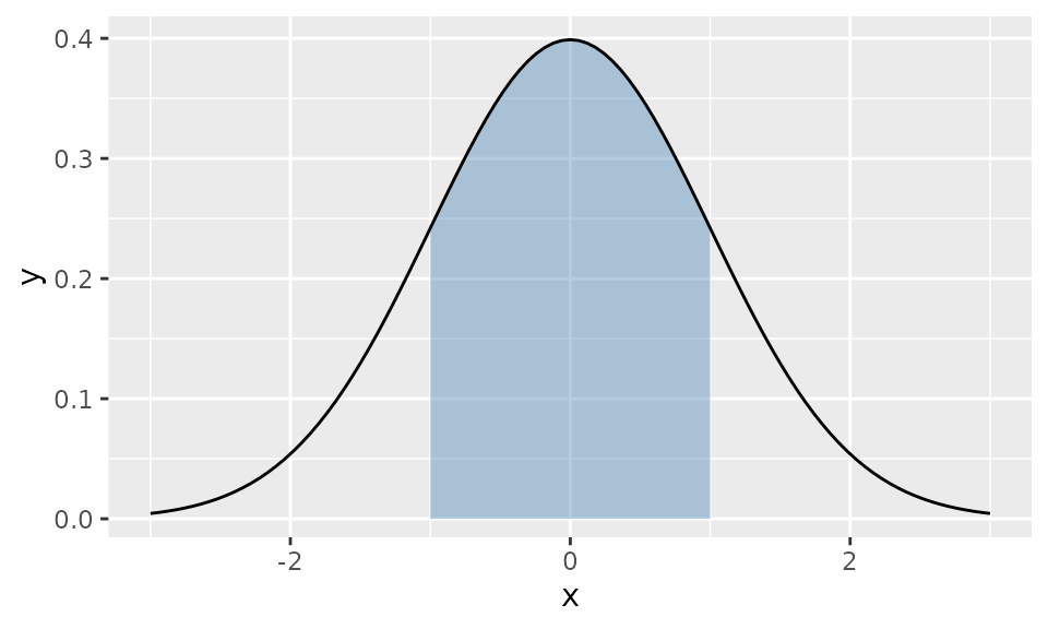
Shade a specific interval:

ggplot() +
  geom_function_1d_1d(
    fun = dnorm, xlim = c(-3, 3),
    shade_from = -1, shade_to = 1, fill = "steelblue"
  )

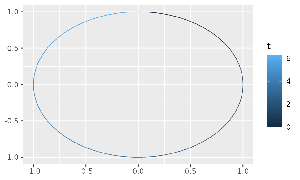
1D to 2D: Parametric Curves

Map a scalar parameter to a 2D path using tlim to set the parameter range:

f <- function(t) c(sin(t), cos(t))
ggplot() +
  geom_function_1d_2d(fun = f, tlim = c(0, 2 * pi))

2D to 1D: Scalar Fields

Visualize $f: \mathbb{R}^2 \to \mathbb{R}$ as a raster:

f_gaussian <- function(v) exp(-(v[1]^2 + v[2]^2) / 2)

ggplot() +
  geom_function_2d_1d(fun = f_gaussian, xlim = c(-3, 3), ylim = c(-3, 3))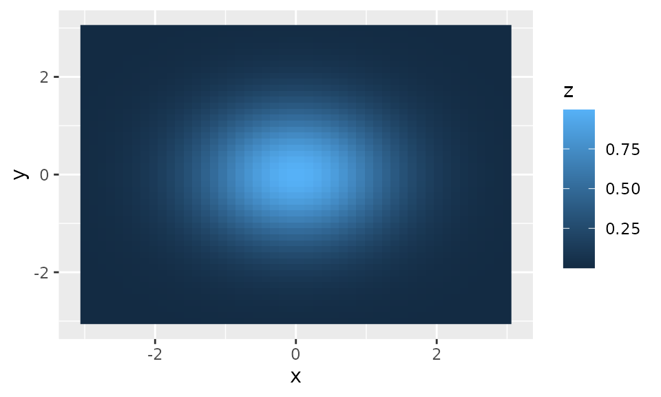

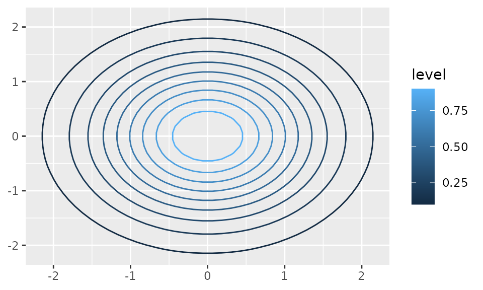
Or as contour lines:

ggplot() +
  geom_function_2d_1d(
    fun = f_gaussian, xlim = c(-3, 3), ylim = c(-3, 3),
    type = "contour"
  )

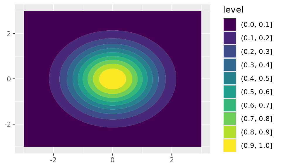
Or as filled contours:

ggplot() +
  geom_function_2d_1d(
    fun = f_gaussian, xlim = c(-3, 3), ylim = c(-3, 3),
    type = "contour_filled"
  )

2D to 2D: Vector Fields

Visualize vector fields as short arrows at each grid point (the default, type = "vector"):

f_rotation <- function(u) c(-u[2], u[1])
ggplot() +
  geom_function_2d_2d(fun = f_rotation, xlim = c(-1, 1), ylim = c(-1, 1))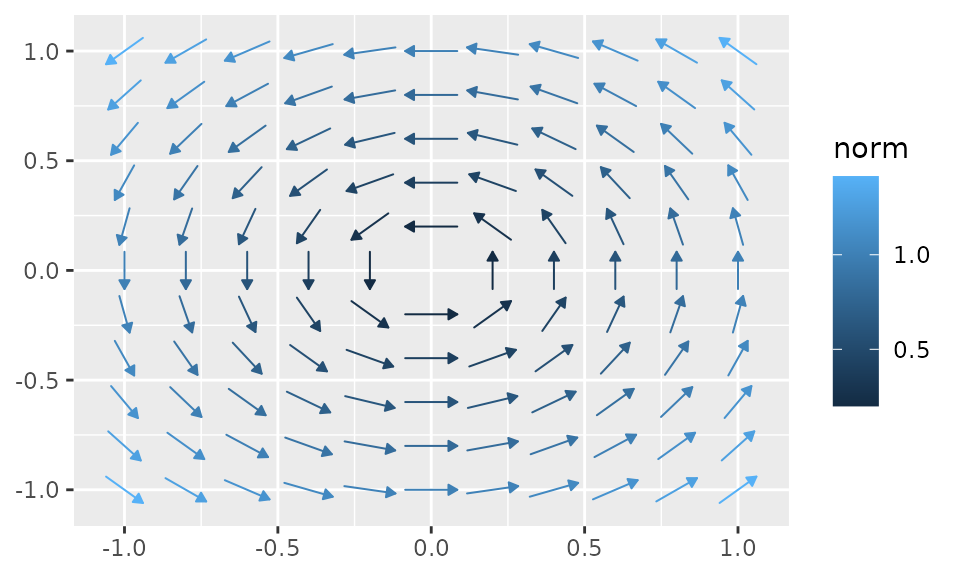

Or as integral-curve streamlines with type = "stream":

ggplot() +
  geom_function_2d_2d(fun = f_rotation, xlim = c(-1, 1), ylim = c(-1, 1),
    type = "stream")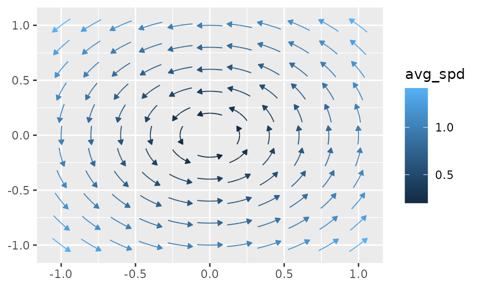

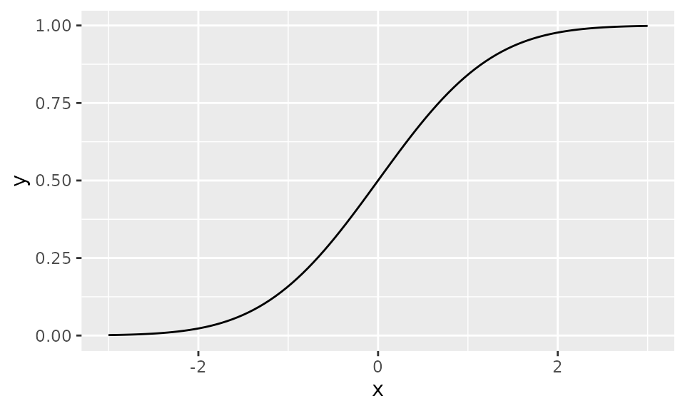
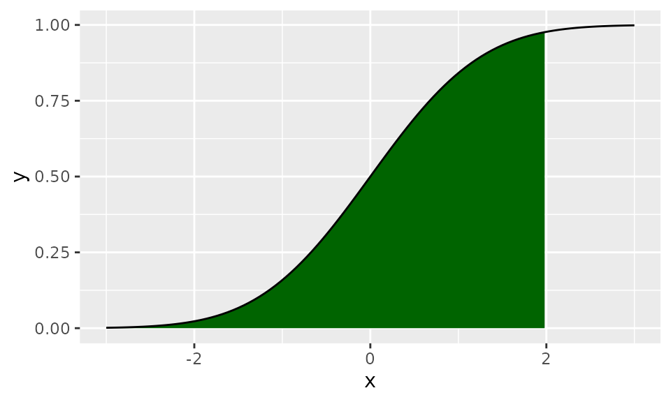
Probability Distribution Family

PDF with Shading

ggplot() +
  geom_pdf(fun = dnorm, xlim = c(-3, 3), p = 0.975, fill = "tomato")

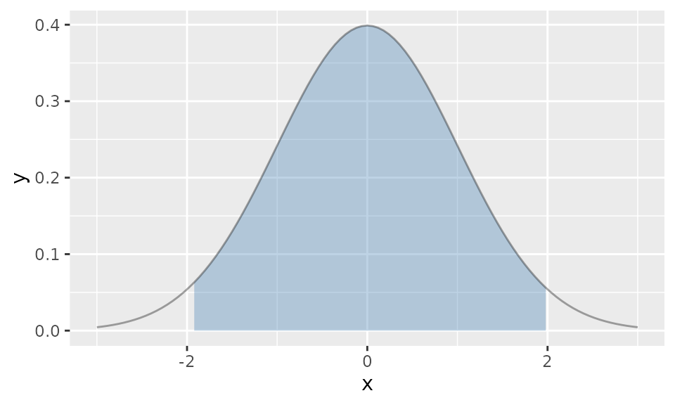
Two-sided shading (e.g., middle 95%):

ggplot() +
  geom_pdf(
    fun = dnorm, xlim = c(-3, 3),
    p_lower = 0.025, p_upper = 0.975, fill = "steelblue"
  )

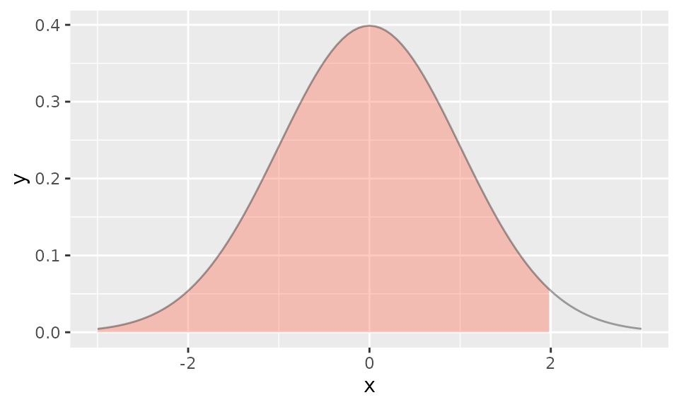
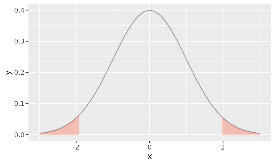
Shade the tails instead (outside):

ggplot() +
  geom_pdf(
    fun = dnorm, xlim = c(-3, 3),
    p_lower = 0.025, p_upper = 0.975, shade_outside = TRUE, fill = "tomato"
  )

CDF

ggplot() +
  geom_cdf(fun = pnorm, xlim = c(-3, 3))

With shading below a quantile:

ggplot() +
  geom_cdf(fun = pnorm, xlim = c(-3, 3), p = 0.975, fill = "darkgreen")

PMF (Lollipop)

ggplot() +
  geom_pmf(fun = dbinom, xlim = c(0, 10), args = list(size = 10, prob = 0.3))

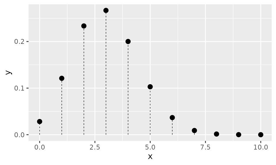
Tail shading with p and HDR shading with shade_hdr work the same way as in geom_pdf():

ggplot() +
  geom_pmf(fun = dbinom, xlim = c(0, 10), args = list(size = 10, prob = 0.5), p = 0.8)

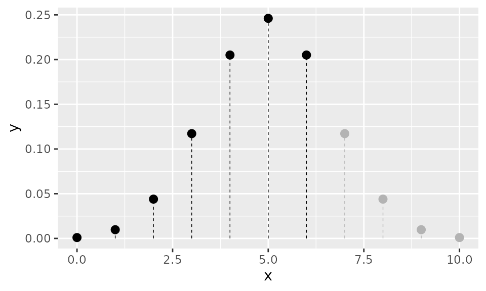
ggplot() +
  geom_pmf(fun = dbinom, xlim = c(0, 10), args = list(size = 10, prob = 0.3),
    shade_hdr = 0.7)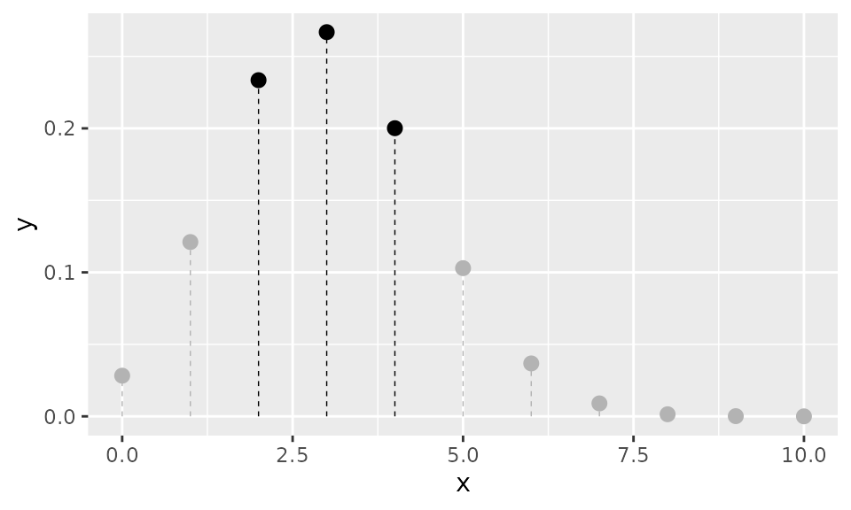

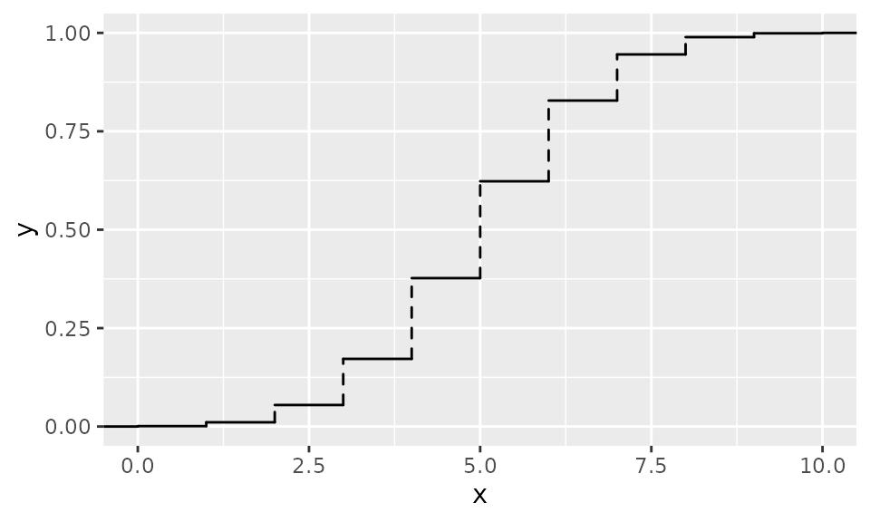
Quantile Function

ggplot() +
  geom_qf(fun = qnorm, args = list(mean = 0, sd = 1))

Discrete CDF (Step Function)

geom_cdf_discrete() renders a discrete CDF as a right-continuous step function with dashed vertical jumps and open/closed endpoint circles:

ggplot() +
  geom_cdf_discrete(
    pmf_fun = dbinom, xlim = c(0, 10), args = list(size = 10, prob = 0.5)
  )

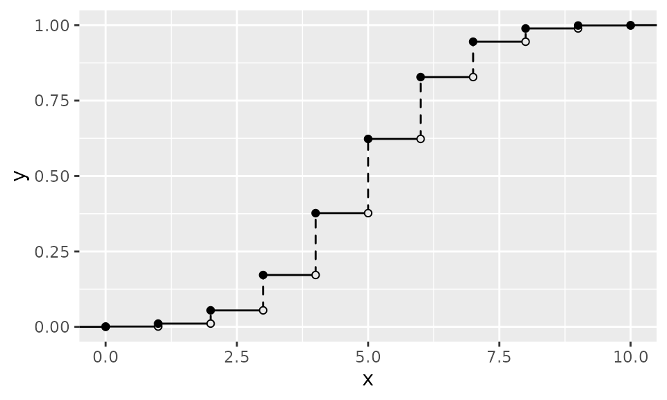
Use show_points = FALSE or show_vert = FALSE to suppress circles or jump lines:

ggplot() +
  geom_cdf_discrete(
    pmf_fun = dbinom, xlim = c(0, 10), args = list(size = 10, prob = 0.5),
    show_points = FALSE
  )

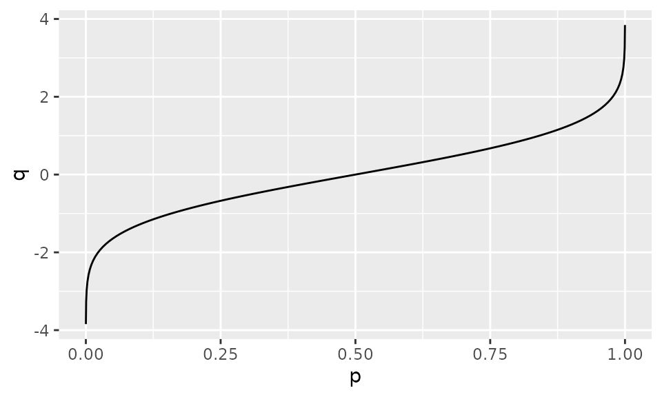
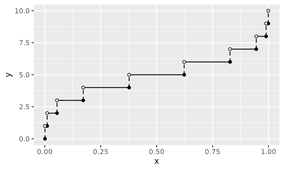
Discrete Quantile Function (Step Function)

geom_qf_discrete() renders the inverse of the discrete CDF as a left-continuous step function on $[0, 1]$, with closed circles at the bottom of each jump and open circles at the top:

ggplot() +
  geom_qf_discrete(
    pmf_fun = dbinom, xlim = c(0, 10), args = list(size = 10, prob = 0.5)
  )

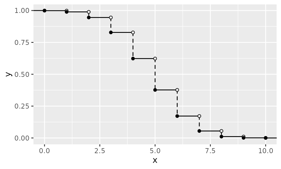
Discrete Survival Function (Step Function)

geom_survival_discrete() renders the discrete survival function $S(x) = 1 - F(x) = P(X > x)$ as a right-continuous step function with the same visual conventions as geom_cdf_discrete():

ggplot() +
  geom_survival_discrete(
    pmf_fun = dbinom, xlim = c(0, 10), args = list(size = 10, prob = 0.5)
  )

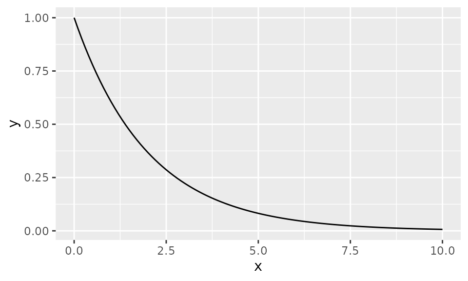
Survival Function

ggplot() +
  geom_survival(fun = pexp, xlim = c(0, 10), args = list(rate = 0.5))

Hazard Function

The exponential distribution has a constant hazard rate:

ggplot() +
  geom_hf(
    pdf_fun = dexp, cdf_fun = pexp,
    xlim = c(0.01, 10), args = list(rate = 0.5)
  )