Lesson 23: Fixed, Random and Mixed Effects

Break!

The New York Marlins youth baseball team and two coaches posed at home plate in front of fall trees.

The Turner family selfie in the stands at Williamsport.

Reese winding up to throw a softball while an Army softball player cheers behind her at Williamsport.

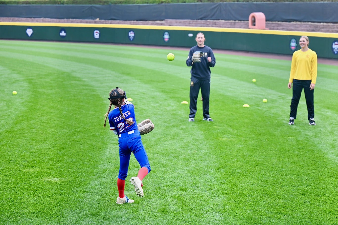
Reese in a blue uniform throwing a softball to two college softball players on the outfield grass at Williamsport.

Reese leaping over small hurdles on the outfield grass at Williamsport.

Cal with a glove standing next to a player on the field at Williamsport.


Calendar

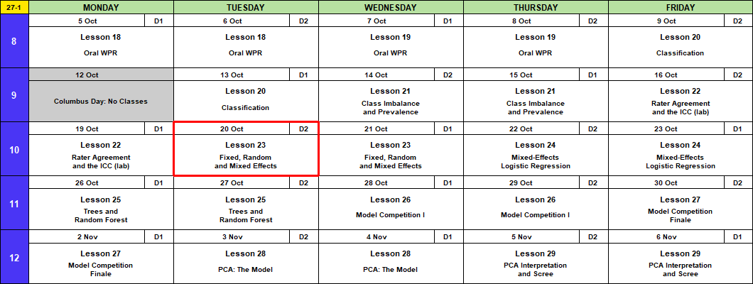
Calendar for 5 October to 6 November with a red box around Tuesday 20 October, Lesson 23, Fixed, Random and Mixed Effects.


Admin

  • This lesson
  • Lesson 27
    • Block 3 quiz (Lessons 20 to 23)
    • Memo 4 due in class, hard copy
  • Capstone Milestone 2: methodology and preliminary results. Due 2359 Friday 13 November, 60 points.
    • 2 to 4 pages that motivate and defend your method, with a short look at results
    • A plebe in MA103 should understand at least 80% of it
  • Capstone final presentation. Lessons 37 and 38, 3 to 8 December, 100 points.
  • I’m here through Lesson 29, 6 November.

What We Did: Lesson 22

  • A rater is a classifier with no truth column, so agreement replaces accuracy.
  • Kappa removes chance agreement. It falls as prevalence moves to an extreme. PABAK puts the prevalence at half.
  • The ICC is the share of the variance that is rep to rep, from a two-way ANOVA with graders as blocks.
  • Grader D never called a no rep. Kappa and the grader effect found him. PABAK did not.

What We’re Doing: Lesson 23

Objectives

  • Frame. A factor is fixed when its levels are the only ones you care about and random when they are a sample of many.
  • Apply. Fit a random-intercept model with lme4 and recover the ICC from its variance components.
  • Mean. A random intercept shrinks a small group toward the overall mean. The ICC is the correlation between two observations in the same group.
  • Communicate. Explain what a company effect means when the companies are a sample.

Reading

None.


The AFT Data

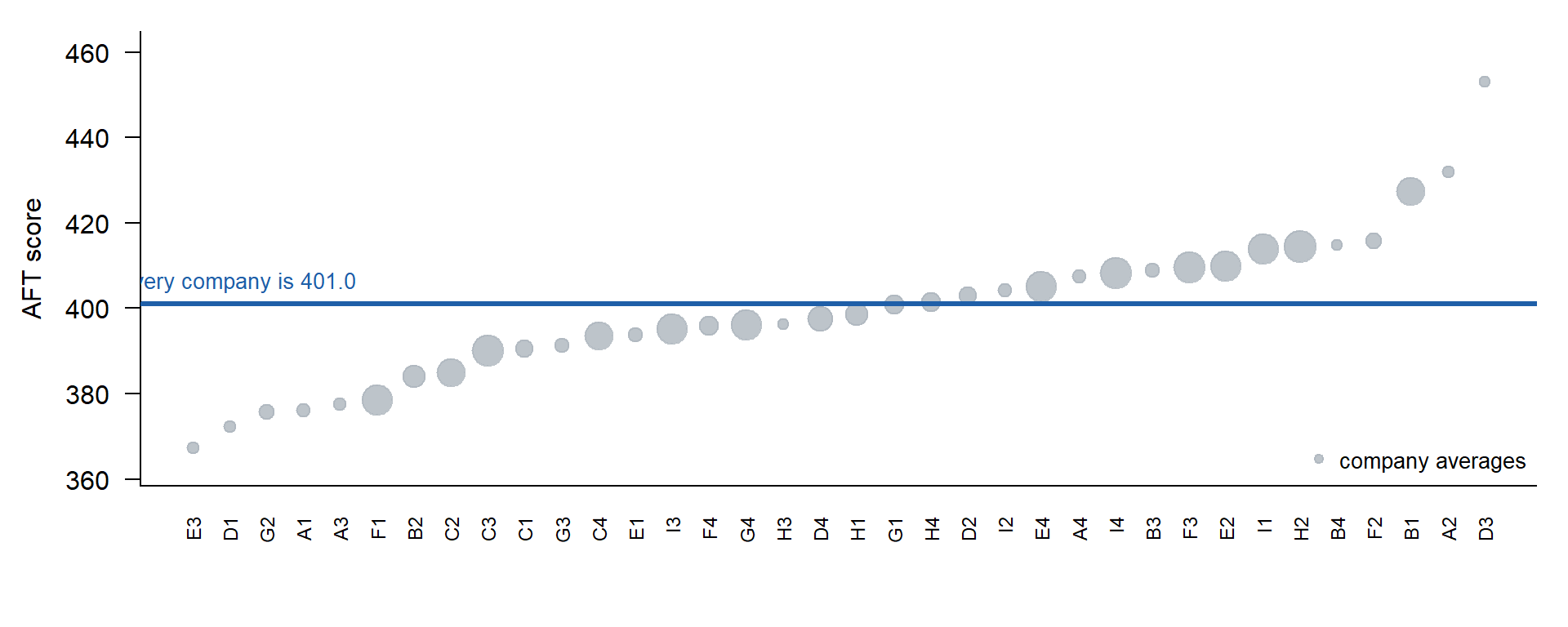
Fall Army Fitness Test (AFT) results reported so far. Some companies have tested most cadets, some only a handful.

  • company: A1 to I4, 36 companies
  • score: AFT total, 0 to 500
  • 1,684 cadets. 4 to 120 per company.
aft <- read.csv("data/L23_aft_companies.csv")
head(aft)
  company score
1      A1   353
2      A1   329
3      A1   443
4      A1   347
5      A1   387
6      A1   386
table(aft$company)    # cadets tested per company

 A1  A2  A3  A4  B1  B2  B3  B4  C1  C2  C3  C4  D1  D2  D3  D4  E1  E2  E3  E4 
  8   5   6   8  80  45  10   4  20  80 110  80   5  20   4  60  10 100   5 100 
 F1  F2  F3  F4  G1  G2  G3  G4  H1  H2  H3  H4  I1  I2  I3  I4 
100  15 110  30  30  12  10 100  45 120   4  30 100   8 100 110 

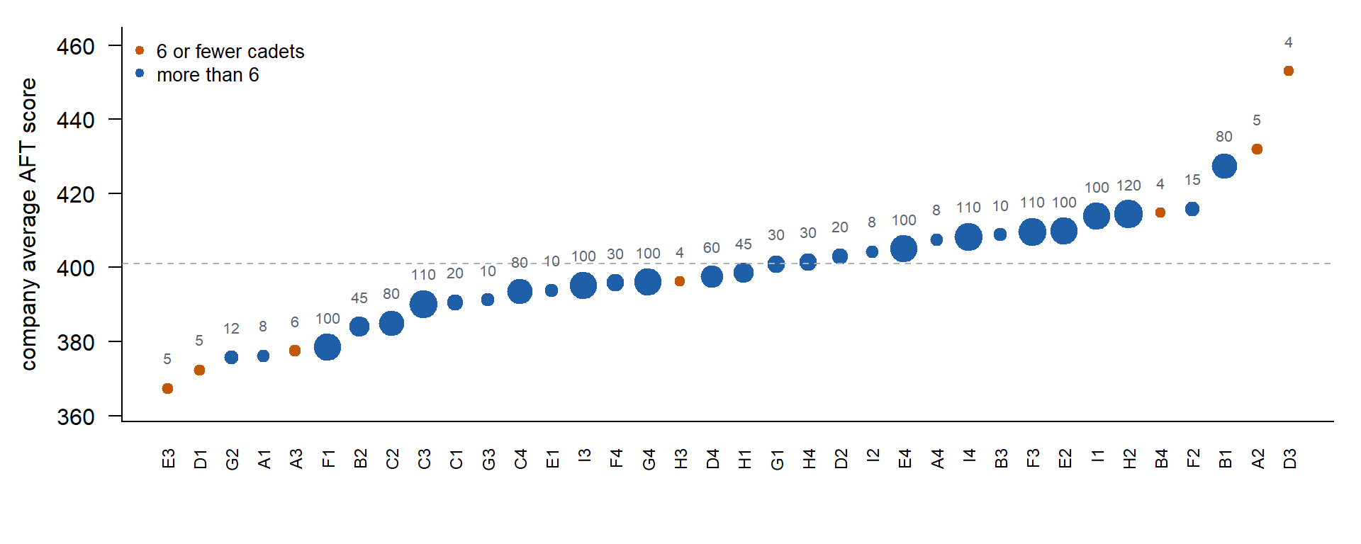
The number over each dot is how many cadets tested.

The commander’s question: which company is the most fit?

The highest and lowest dots are orange. Fitness or luck? Three ways to model it.


Model 1: No Company Effect

\[y_{ij} = \mu + \varepsilon_{ij}, \qquad \varepsilon_{ij} \sim N(0, \sigma^2)\]

  • \(y_{ij}\): cadet \(i\) in company \(j\)
  • \(\mu\): the overall average
  • \(\varepsilon_{ij}\): how far cadet \(i\) sits from \(\mu\)
fit1 <- lm(score ~ 1, data = aft)
summary(fit1)

Call:
lm(formula = score ~ 1, data = aft)

Residuals:
     Min       1Q   Median       3Q      Max 
-140.952  -28.952    0.048   29.048   99.048 

Coefficients:
            Estimate Std. Error t value Pr(>|t|)    
(Intercept)  400.952      1.038   386.4   <2e-16 ***
---
Signif. codes:  0 '***' 0.001 '**' 0.01 '*' 0.05 '.' 0.1 ' ' 1

Residual standard error: 42.58 on 1683 degrees of freedom

  • One parameter. Every company gets 401.0.
  • Answer to the commander: they are all the same. The plot says they are not.

Predicting a Cadet

\[\hat y_{ij} = \hat\mu\]

  • A cadet in D3: \(401.0\)
  • A cadet in H2: \(401.0\)
  • A cadet in J5, a new company: \(401.0\)
predict(fit1, data.frame(company = c("D3", "H2", "J5")))   # J5 is a new company
       1        2        3 
400.9519 400.9519 400.9519 

Model 2: Fixed Company Effect

Lesson 13: ANOVA is regression with indicators.

\[y_{ij} = \beta_0 + \beta_j + \varepsilon_{ij}\]

  • \(\beta_0\): company A1’s average (the baseline)
  • \(\beta_j\): how far company \(j\) sits from A1, one dummy per company
fit2 <- lm(score ~ company, data = aft)
summary(fit2)

Call:
lm(formula = score ~ company, data = aft)

Residuals:
     Min       1Q   Median       3Q      Max 
-124.800  -26.736   -1.286   27.487  121.590 

Coefficients:
            Estimate Std. Error t value Pr(>|t|)    
(Intercept)  376.250     14.505  25.939  < 2e-16 ***
companyA2     55.750     23.389   2.384 0.017256 *  
companyA3      1.250     22.157   0.056 0.955018    
companyA4     31.375     20.513   1.529 0.126335    
companyB1     51.250     15.213   3.369 0.000772 ***
companyB2      7.706     15.742   0.489 0.624555    
companyB3     32.550     19.461   1.673 0.094596 .  
companyB4     38.500     25.124   1.532 0.125611    
companyC1     14.350     17.163   0.836 0.403212    
companyC2      8.825     15.213   0.580 0.561933    
companyC3     13.923     15.023   0.927 0.354198    
companyC4     17.325     15.213   1.139 0.254944    
companyD1     -3.850     23.389  -0.165 0.869272    
companyD2     26.750     17.163   1.559 0.119281    
companyD3     76.750     25.124   3.055 0.002288 ** 
companyD4     21.267     15.442   1.377 0.168636    
companyE1     17.550     19.461   0.902 0.367286    
companyE2     33.550     15.074   2.226 0.026172 *  
companyE3     -8.850     23.389  -0.378 0.705193    
companyE4     28.770     15.074   1.909 0.056492 .  
companyF1      2.160     15.074   0.143 0.886078    
companyF2     39.617     17.961   2.206 0.027546 *  
companyF3     33.486     15.023   2.229 0.025951 *  
companyF4     19.550     16.325   1.198 0.231265    
companyG1     24.650     16.325   1.510 0.131247    
companyG2     -0.500     18.726  -0.027 0.978702    
companyG3     14.950     19.461   0.768 0.442470    
companyG4     19.800     15.074   1.314 0.189196    
companyH1     22.283     15.742   1.416 0.157095    
companyH2     38.092     14.981   2.543 0.011091 *  
companyH3     20.000     25.124   0.796 0.426110    
companyH4     25.217     16.325   1.545 0.122619    
companyI1     37.550     15.074   2.491 0.012836 *  
companyI2     28.125     20.513   1.371 0.170544    
companyI3     18.950     15.074   1.257 0.208890    
companyI4     32.123     15.023   2.138 0.032648 *  
---
Signif. codes:  0 '***' 0.001 '**' 0.01 '*' 0.05 '.' 0.1 ' ' 1

Residual standard error: 41.03 on 1648 degrees of freedom
Multiple R-squared:  0.09084,   Adjusted R-squared:  0.07153 
F-statistic: 4.704 on 35 and 1648 DF,  p-value: < 2.2e-16
  • 36 parameters. Each company’s estimate is its own average: the dots in the first plot.
  • Answer to the commander: D3, at 453.0, on 4 cadets.
  • The highest and lowest companies are the small ones. A 4-cadet average is off by about 21 points by luck alone; real companies differ by about 11.
  • D3’s 4 cadets count as much as H2’s 120.

Predicting a Cadet

\[\hat y_{ij} = \hat\beta_0 + \hat\beta_j\]

  • A cadet in D3: \(376.25 + 76.75 = 453.0\)
  • A cadet in H2: \(376.25 + 38.09 = 414.3\)
  • A cadet in J5, a new company: no \(\hat\beta_{J5}\), so no prediction
predict(fit2, data.frame(company = c("D3", "H2")))
       1        2 
453.0000 414.3417 
try(predict(fit2, data.frame(company = "J5")))   # J5 is a new company
Error in model.frame.default(Terms, newdata, na.action = na.action, xlev = object$xlevels) : 
  factor company has new level J5

Model 3: Random Company Effect

Model 2 trusts 4 cadets as much as 120 and says nothing about J5. Model 3 fixes both with one new assumption about the company effects:

  • Model 2: 36 unrelated numbers. Each company’s effect comes only from its own cadets.
  • Model 3: all 36 come from one normal distribution. Companies tell you about each other.
Differences between companies Differences between cadets in a company
Model 2 35 separate \(\beta_j\), no variance one variance, \(\sigma^2\)
Model 3 one variance, \(\sigma^2_u\) one variance, \(\sigma^2\)

\[y_{ij} = \mu + u_j + \varepsilon_{ij}, \qquad u_j \sim N(0, \sigma^2_u), \qquad \varepsilon_{ij} \sim N(0, \sigma^2)\]

  • \(\mu\): the overall average
  • \(u_j\): how far company \(j\) sits from \(\mu\) (like Model 2’s \(\beta_j\), but measured from \(\mu\), not A1)
  • \(\sigma^2_u\): how much companies differ
  • \(\sigma^2\): the variance left over after accounting for company

Fitting It: lmer

lmer() from the lme4 package: linear mixed-effects regression. Same formula as lm(), plus random effects.

Piece of the formula Means Effect
score ~ 1 one overall average, \(\mu\) Fixed: one number, estimated directly (\(\hat\mu\)). Fixed effects in the summary.
(1 | company) an intercept (\(1\)) for each company, drawn from \(N(0, \sigma^2_u)\) Random: estimate their spread (\(\hat\sigma^2_u\)), then predict each \(u_j\). Random effects in the summary.
library(lme4)
fit3 <- lmer(score ~ 1 + (1 | company), data = aft)
summary(fit3)
Linear mixed model fit by REML ['lmerMod']
Formula: score ~ 1 + (1 | company)
   Data: aft

REML criterion at convergence: 17330.1

Scaled residuals: 
     Min       1Q   Median       3Q      Max 
-2.99943 -0.64960 -0.03483  0.67039  2.90049 

Random effects:
 Groups   Name        Variance Std.Dev.
 company  (Intercept)  125.6   11.21   
 Residual             1685.3   41.05   
Number of obs: 1684, groups:  company, 36

Fixed effects:
            Estimate Std. Error t value
(Intercept)  399.704      2.374   168.3
  • Random effects: the two variances; read the Variance column (Std.Dev. is its square root). company is \(\hat\sigma^2_u = 125.6\). Residual is \(\hat\sigma^2 = 1685.3\).
  • Fixed effects: (Intercept) is \(\hat\mu = 399.7\).
  • 3 parameters: \(\mu\), \(\sigma^2_u\), \(\sigma^2\).

The Model 3 Formula

Like Models 1 and 2, predict a cadet by dropping \(\varepsilon_{ij}\) (it averages 0):

\[\hat y_{ij} = \hat\mu + \hat u_j = \hat\mu + w_j\,(\bar y_j - \hat\mu)\]

The overall average \(\hat\mu = 399.7\), plus a share \(w_j\) of the company’s gap from it. Multiply out and regroup: \(\hat\mu + w_j\bar y_j - w_j\hat\mu = w_j\,\bar y_j + (1 - w_j)\,\hat\mu\), a blend of the company’s own average and the overall average.

\[w_j = \frac{n_j}{n_j + \lambda}, \qquad \lambda = \frac{\hat\sigma^2}{\hat\sigma^2_u} = \frac{1685.3}{125.6} = 13.4\]

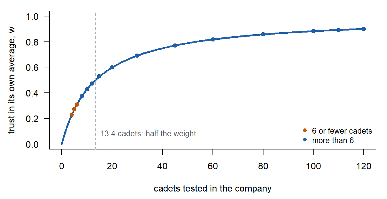
  • \(w_j\): the trust in the company’s own average, between 0 (ignore it, Model 1) and 1 (take all of it, Model 2). More cadets (\(n_j\)), more trust.
  • \(\lambda\): cadet noise (Residual) over how much companies really differ (company), both from the summary. Big when cadets vary a lot or companies barely differ, small when companies really differ.
  • Here \(\lambda = 13.4\): a company needs about 13 cadets before its own average gets half the weight.

The \(\hat u_j\). Lesson 8’s ridge regression. lmer picks the \(u_j\) that minimize

\[\underbrace{\sum_{i,j} (y_{ij} - \mu - u_j)^2}_{\text{fit the cadets}} \;+\; \underbrace{\lambda \sum_j u_j^2}_{\text{penalty: keep each } u_j \text{ near } 0}\]

  • First part: least squares, same as lm. Alone, it gives Model 2: each company its own average.
  • Second part: a ridge penalty that pulls every \(u_j\) toward 0, the overall average. \(\lambda\) sets how hard.

Solve for one company. Only company \(j\)’s cadets involve \(u_j\):

\[f(u_j) = \sum_{i=1}^{n_j} (y_{ij} - \mu - u_j)^2 + \lambda u_j^2\]

1. Take the derivative.

\[f'(u_j) = -2\sum_{i=1}^{n_j} (y_{ij} - \mu - u_j) + 2\lambda u_j\]

2. Set it to 0. The sum of \(n_j\) cadets’ scores is \(n_j \bar y_j\), so \(\sum_i (y_{ij} - \mu - u_j) = n_j(\bar y_j - \mu - u_j)\):

\[n_j(\bar y_j - \mu - u_j) = \lambda u_j\]

3. Solve for \(u_j\).

\[n_j(\bar y_j - \mu) = (n_j + \lambda)\,u_j \quad\Rightarrow\quad \hat u_j = \frac{n_j}{n_j + \lambda}\,(\bar y_j - \hat\mu)\]

The trust \(w_j\) times the raw gap, as above.

  • \(\lambda = 0\), no penalty: \(w_j = 1\), \(\hat u_j\) is the whole raw gap. Model 2.
  • \(\lambda\) huge: \(w_j \to 0\), \(\hat u_j \to 0\). Every company is the overall average. Model 1.
  • Model 3 sits between, and \(\lambda\) decides where.

Why \(\lambda\) is the variance ratio. Lesson 8 tuned \(\lambda\) by cross-validation. Here the assumption \(u_j \sim N(0, \sigma^2_u)\) sets it. Model 3’s two assumptions, written as \(-2 \log\) density (constants dropped), have two pieces:

\[\underbrace{\frac{1}{\sigma^2}\sum_{i,j}(y_{ij} - \mu - u_j)^2}_{\text{cadets: } \varepsilon \sim N(0, \sigma^2)} + \underbrace{\frac{1}{\sigma^2_u}\sum_j u_j^2}_{\text{companies: } u_j \sim N(0, \sigma^2_u)}\]

Multiply by \(\sigma^2\): the ridge objective with \(\lambda = \sigma^2 / \sigma^2_u\). Ridge had no rule for \(\lambda\). This assumption gives one.

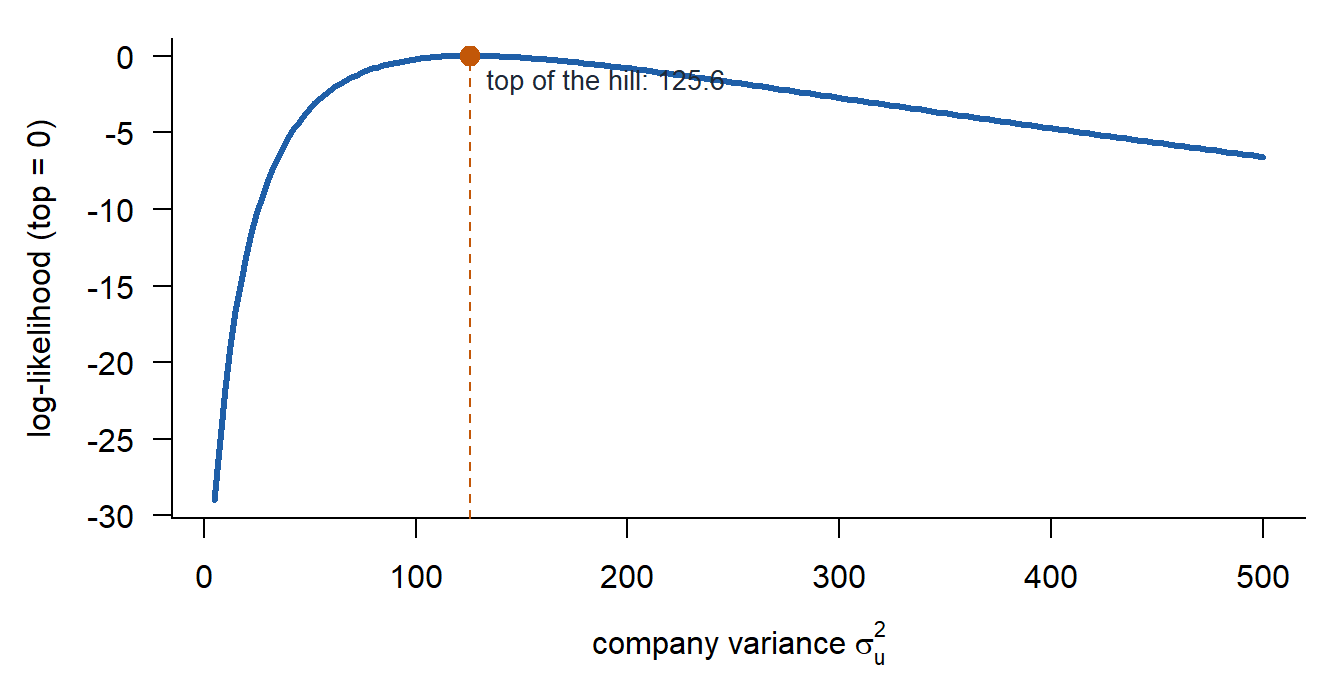
How lmer finds the two variances. By maximum likelihood, with calculus, like Lesson 9’s logistic regression.

1. Write down how likely the data are for any values of the two variances. Company \(j\)’s average has variance \(v_j = \sigma^2_u + \sigma^2 / n_j\): real company spread plus the luck of \(n_j\) cadets. The maximum likelihood (ML) log-likelihood:

\[\ell(\mu, \sigma^2_u, \sigma^2) = -\frac{1}{2}\sum_j \left[ (n_j - 1)\log\sigma^2 + \frac{SS_j}{\sigma^2} + \log v_j + \frac{(\bar y_j - \mu)^2}{v_j} \right] + \text{const}\]

\(SS_j\): the sum of squares of cadets around their own company average.

2. Take the derivative and set it to 0.

\[\frac{\partial \ell}{\partial \sigma^2_u} = -\frac{1}{2}\sum_j \left[ \frac{1}{v_j} - \frac{(\bar y_j - \mu)^2}{v_j^2} \right] = 0\]

3. No closed-form answer. \(\sigma^2_u\) sits inside every \(v_j\), and each company has its own \(n_j\). You cannot solve it by hand. The computer climbs the hill, as glm did in Lesson 9. lmer uses REML, a version of maximum likelihood with a small correction for estimating \(\mu\): it adds \(-\tfrac{1}{2}\log \sum_j 1/v_j\) to \(\ell\). The hill below is REML.

4. Read off the top. \(\hat\sigma^2_u = 125.6\) and \(\hat\sigma^2 = 1685.3\).
D3: \(n_j = 4\), \(\bar y_j = 453.0\).

\[w = \frac{4}{4 + 13.4} = 0.23, \qquad \hat y = 399.7 + 0.23\,(453.0 - 399.7) = 411.9\]

H2: \(n_j = 120\), \(\bar y_j = 414.3\).

\[w = \frac{120}{120 + 13.4} = 0.90, \qquad \hat y = 399.7 + 0.90\,(414.3 - 399.7) = 412.9\]

  • D3: 4 cadets, \(w = 0.23\). Keeps 23% of its gap.
  • H2: 120 cadets, \(w = 0.90\). Keeps 90% of its gap.

A new company, J5: no cadets, so no gap to trust. \(\hat u_{J5} = 0\) and \(\hat y = 399.7\).

Why shrink? A 4-cadet average is off by about 20.5 points from luck alone; companies really differ by about 11.2. Mostly luck, so D3 keeps 23% of its gap. H2’s 120 cadets: luck about 3.7, so it keeps 90%. The larger the sample, the more we trust the company average and the less we shrink.

The same \(w_j\) two ways. Divide top and bottom by \(n_j\) and put in \(\lambda = \hat\sigma^2 / \hat\sigma^2_u\): real spread over real spread plus luck.

\[w_j = \frac{n_j}{n_j + \lambda} = \frac{\hat\sigma^2_u}{\hat\sigma^2_u + \hat\sigma^2 / n_j}\]

\[w_{D3} = \frac{4}{4 + 13.4} = \frac{11.2^2}{11.2^2 + 20.5^2} = 0.23\]

fixef(fit3)                                            # mu-hat
(Intercept) 
   399.7035 
ranef(fit3)$company[c("D3", "H2"), , drop = FALSE]     # u-hat = y-hat minus mu-hat
   (Intercept)
D3    12.23671
H2    13.16557
predict(fit3, data.frame(company = c("D3", "H2", "J5")), allow.new.levels = TRUE)   # J5 is new: allow.new.levels sets u-hat = 0 (Model 2 errors)
       1        2        3 
411.9403 412.8691 399.7035 
  • ranef gives \(\hat u_j = \hat y - \hat\mu\): 12.2 for D3, 13.2 for H2.
  • predict matches the hand values, and J5 gets \(\hat\mu\).

Shrinkage

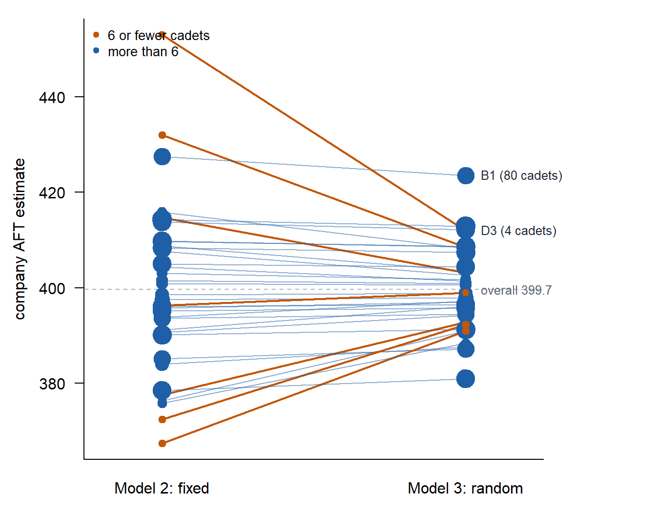
  • Small companies get pulled toward the overall average. Large companies barely move.
  • This is shrinkage.
Rank Model 2: company (cadets) Estimate Model 3: company (cadets) Estimate
1 D3 (4) 453.0 B1 (80) 423.5
2 A2 (5) 432.0 H2 (120) 412.9
3 B1 (80) 427.5 I1 (100) 412.1
4 F2 (15) 415.9 D3 (4) 411.9
5 B4 (4) 414.8 F3 (110) 408.6

Answer to the commander: B1. 80 cadets, a high average that holds up.


Side by Side

R Parameters D3 (4 cadets) H2 (120 cadets) J5 (new company)
Model 1: no company effect lm(score ~ 1) 1 401.0 401.0 401.0
Model 2: fixed company effect lm(score ~ company) 36 453.0 414.3 nothing to say
Model 3: random company effect lmer(score ~ 1 + (1 | company)) 3 411.9 412.9 399.7

How Much Does Company Matter? The ICC

From Model 3’s two variances, \(\hat\sigma^2_u = 125.6\) (company) and \(\hat\sigma^2 = 1685.3\) (cadet):

ImportantThe ICC

\[\text{ICC} = \frac{\hat\sigma^2_u}{\hat\sigma^2_u + \hat\sigma^2} = \frac{125.6}{125.6 + 1685.3} = 0.069\]

Intraclass correlation coefficient (ICC): Lesson 22’s share of variance from the groups, now read straight off lmer’s two variances.

  • 0: the company tells you nothing. Every company looks the same.
  • 1: everyone in a company scores the same. All the variation is company to company.
  • 7% of the variation in a cadet’s score comes from the company. The rest is cadet to cadet.
  • Also a correlation: two cadets in the same company have scores correlated at 0.07.
  • So cadets in a company are not independent. Model 1 assumes they are, so its standard errors are too small.

Two cadets in the same company share \(u_j\):

\[y_{1j} = \mu + u_j + \varepsilon_{1j}, \qquad y_{2j} = \mu + u_j + \varepsilon_{2j}\]

\[\text{Cor}(y_{1j}, y_{2j}) = \frac{\text{Cov}(y_{1j}, y_{2j})}{\text{Var}(y_{1j})} = \frac{\sigma^2_u}{\sigma^2_u + \sigma^2} = \text{ICC}\]

The ICC Sets the Pull

\[\lambda = \frac{\hat\sigma^2}{\hat\sigma^2_u} = \frac{1 - \text{ICC}}{\text{ICC}} = \frac{1 - 0.069}{0.069} = 13.4\]


Tell the Commander

Company matters, but not much: 7% of the variation in AFT scores is company to company, and most company averages sit within about 22 points of 400. Do not rank companies on a handful of scores. D3 tops the raw board on 4 cadets, and its estimate drops to 412 once you account for how little 4 scores tell you. On the evidence so far, B1 is the most fit company.


Fixed or Random?

Model 2 treats company as a fixed effect. Model 3 treats it as a random effect.

Fixed Random
The levels the only ones you care about a sample of many
Companies these 36 companies are all that matter these 36 stand in for companies in general, including J5, a company not in the data
The question is this level different? how much do levels vary?
Companies is D3 better than B1? how much do companies differ?
Estimates one effect per level one variance
Companies 36 company averages \(\hat\sigma^2_u = 125.6\), companies differ by about 11 points (SD)
Small groups taken at face value pulled toward the overall average
Pick it when few levels, every one well sampled many levels, or some thinly sampled, even when you want to rank them

Mixed model: some effects fixed, some random. Model 3 is already one: \(\mu\) fixed (the Fixed effects block), company random. Lesson 24 adds fixed predictors.

Your Turn

Fixed or random?

  1. Three fertilizer brands. You will buy one.
  2. 12 recruiting stations sampled from the hundreds in USAREC.
  3. Day 1 and Day 2 sections of MA376.
  4. 30 patients in a drug trial, each measured every week.
  5. The four AFT test sites at West Point. The Master of the Sword wants to know which one scores low.
  6. 20 Army units chosen for a survey on retention.
  1. Fixed. You care about these three.
  2. Random. The stations stand in for all of them.
  3. Fixed. There are only two days.
  4. Random. The patients stand in for future patients.
  5. Fixed. The question is about these four sites.
  6. Random. The units stand in for the Army.

Practice: Radon in Minnesota

Radon is a radioactive gas that seeps into basements from the ground. The state of Minnesota tested homes in every county it could reach.

  • county: 85 Minnesota counties
  • log_radon: radon level on the log scale (log of picocuries per liter)
  • 919 homes. 1 to 116 per county. 11 counties tested 2 homes or fewer.
  • Source: Gelman and Hill (2007), Data Analysis Using Regression and Multilevel/Hierarchical Models.
library(tidyverse)
radon <- read_csv("data/L23_radon_counties.csv", show_col_types = FALSE)

The state’s question: which county has the worst radon?

1. Find each county’s average log_radon and number of homes. Which county is highest? Lowest? How many homes did each test?

avg <- radon |>
  group_by(county) |>
  summarise(n = n(), avg = mean(log_radon))

avg |> arrange(desc(avg)) |> slice_head(n = 3)   # highest
# A tibble: 3 × 3
  county            n   avg
  <chr>         <int> <dbl>
1 Lac Qui Parle     2  2.61
2 Murray            1  2.50
3 Wilkin            1  2.24
avg |> arrange(avg) |> slice_head(n = 3)         # lowest
# A tibble: 3 × 3
  county          n   avg
  <chr>       <int> <dbl>
1 Lake            9 0.410
2 Koochiching     7 0.475
3 Waseca          4 0.534

Highest: Lac Qui Parle, 2.61 on 2 homes. Lowest: Lake, 0.41 on 9 homes. The top three tested 2 homes or fewer.

2. Fit Model 2, a fixed county effect. Which county does it call the worst?

rfit2 <- lm(log_radon ~ county, data = radon)
predict(rfit2, tibble(county = "Lac Qui Parle"))
     1 
2.6062 

Lac Qui Parle, at its own average 2.61, on 2 homes.

3. Fit Model 3, a random county effect. Report \(\hat\mu\), \(\hat\sigma^2_u\), \(\hat\sigma^2\) and \(\lambda\).

rfit3 <- lmer(log_radon ~ 1 + (1 | county), data = radon)
summary(rfit3)
Linear mixed model fit by REML ['lmerMod']
Formula: log_radon ~ 1 + (1 | county)
   Data: radon

REML criterion at convergence: 2184.9

Scaled residuals: 
    Min      1Q  Median      3Q     Max 
-4.6881 -0.5883  0.0323  0.6444  3.4186 

Random effects:
 Groups   Name        Variance Std.Dev.
 county   (Intercept) 0.0886   0.2977  
 Residual             0.5869   0.7661  
Number of obs: 919, groups:  county, 85

Fixed effects:
            Estimate Std. Error t value
(Intercept)    1.350      0.047   28.72
  • \(\hat\mu = 1.350\) (Fixed effects)
  • \(\hat\sigma^2_u = 0.0886\) (county variance), \(\hat\sigma^2 = 0.5869\) (Residual variance)
  • \(\lambda = 0.5869 / 0.0886 = 6.6\): a county needs about 7 homes before its own average gets half the weight.

4. Find \(w\) for Lac Qui Parle (2 homes) and St. Louis (116 homes). Use both forms of \(w_j\).

\[w_{\text{Lac Qui Parle}} = \frac{2}{2 + 6.6} = \frac{0.0886}{0.0886 + 0.5869 / 2} = 0.23\]

\[w_{\text{St. Louis}} = \frac{116}{116 + 6.6} = \frac{0.0886}{0.0886 + 0.5869 / 116} = 0.95\]

Lac Qui Parle keeps 23% of its gap. St. Louis keeps 95%.

5. Predict a home in Lac Qui Parle, a home in St. Louis, and a home in a county the state never tested. By hand, then with predict.

\[\hat y_{\text{Lac Qui Parle}} = 1.350 + 0.23\,(2.606 - 1.350) = 1.64\]

\[\hat y_{\text{St. Louis}} = 1.350 + 0.95\,(0.828 - 1.350) = 0.86\]

New county: \(\hat u = 0\), so \(\hat y = \hat\mu = 1.35\).

tibble(county = c("Lac Qui Parle", "St. Louis", "New County")) |>
  mutate(y_hat = predict(rfit3, newdata = pick(county), allow.new.levels = TRUE))
# A tibble: 3 × 2
  county        y_hat
  <chr>         <dbl>
1 Lac Qui Parle 1.64 
2 St. Louis     0.856
3 New County    1.35 

6. Find the ICC. What share of the radon variation is county to county?

\[\text{ICC} = \frac{0.0886}{0.0886 + 0.5869} = 0.131\]

13% of the variation is county to county. The rest is home to home inside a county.

7. List the top five counties under Model 2 and under Model 3. Who drops out, and why?

est <- coef(rfit3)$county |>
  rownames_to_column("county") |>
  as_tibble() |>
  rename(model3 = `(Intercept)`) |>
  left_join(avg, by = "county")

est |> arrange(desc(avg)) |> slice_head(n = 5)      # Model 2: the county's own average
# A tibble: 5 × 4
  county        model3     n   avg
  <chr>          <dbl> <int> <dbl>
1 Lac Qui Parle   1.64     2  2.61
2 Murray          1.50     1  2.50
3 Wilkin          1.47     1  2.24
4 Watonwan        1.63     3  2.24
5 Nicollet        1.66     4  2.18
est |> arrange(desc(model3)) |> slice_head(n = 5)   # Model 3: shrunk
# A tibble: 5 × 4
  county     model3     n   avg
  <chr>       <dbl> <int> <dbl>
1 Blue Earth   1.74    14  1.93
2 Freeborn     1.70     9  1.96
3 Goodhue      1.70    14  1.87
4 Nicollet     1.66     4  2.18
5 Clay         1.66    14  1.81

Every Model 2 top five county tested 4 homes or fewer. Lac Qui Parle, Murray, Wilkin, Watonwan drop out of the Model 3 top five: their high averages rest on a handful of homes. Blue Earth (14 homes) moves to first.

8. Answer the state in two or three plain sentences.

County matters some: 13% of the variation in radon is county to county. Do not rank counties on two or three homes. Lac Qui Parle tops the raw board on 2 homes, but Blue Earth, on 14 homes, has the highest radon that holds up.

9. A state inspector asks, “Is Lac Qui Parle worse than Blue Earth?” Fixed or random?

Random. There are 85 counties, and 11 of them tested 2 homes or fewer. Even to rank them, shrink first. A fixed effect would take Lac Qui Parle’s 2 homes at face value.


ImportantTakeaway
  • Grouped data, three choices: ignore the group, a dummy for each group, or a random intercept.
  • Dummies take every group’s average at face value, so small groups land at the extremes by luck.
  • A random intercept blends each group’s own average with the overall average. Small groups get pulled toward the overall average.
  • Fixed: you care about these levels. Random: the levels are a sample, and you care about how much they vary.
  • The ICC is the share of the variance between groups. It sets the pull.

Before You Leave

Today

  • Three models for grouped data: ignore the group, dummies, random intercept
  • lmer: a blend of each group’s own average and the overall average
  • Shrinkage: small companies pulled to the middle
  • Fixed or random: these levels, or a sample of levels
  • The ICC: the share of the variance between groups

Any questions?


Next Lesson

Lesson 24: Mixed-Effects Logistic Regression

  • Frame. Leads nested in stations: ignore the station, fit a dummy for each, or fit one random intercept.
  • Apply. Fit a logistic model with a station random intercept, compare the three fits, and score and rank the incoming leads.
  • Mean. What shrinkage does to a small station, why the dummies overfit, and why ignoring the station misleads.
  • Communicate. Tell the battalion which stations convert above the rest and how sure you are.