Lesson 26: Two-Proportion z-Test
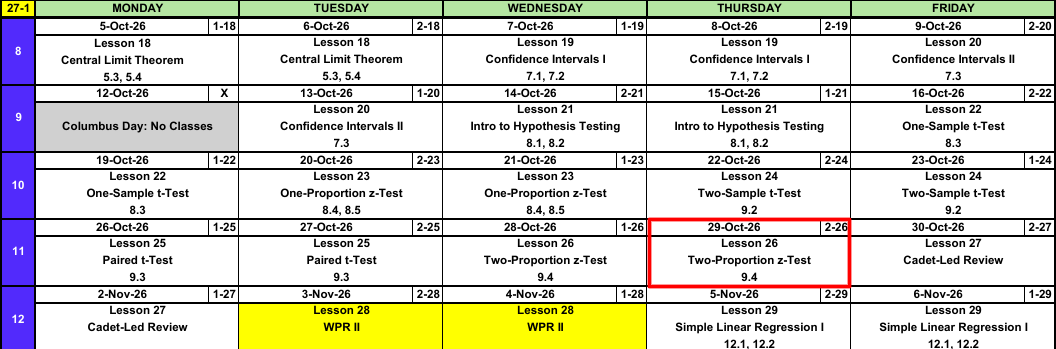
Calendar
Warm-Up
Ruck: Same Cadets
Do new boots lower 12 mile ruck times? Eight randomly selected cadets rucked once in their old boots and once in new boots (hours). Test at \(\alpha = 0.05\).
| Cadet | 1 | 2 | 3 | 4 | 5 | 6 | 7 | 8 |
|---|---|---|---|---|---|---|---|---|
| Old | 3.05 | 2.88 | 3.21 | 2.79 | 3.12 | 2.95 | 3.30 | 2.84 |
| New | 2.94 | 2.85 | 3.06 | 2.80 | 2.98 | 2.87 | 3.15 | 2.76 |
| \(d\) = New \(-\) Old | -0.11 | -0.03 | -0.15 | 0.01 | -0.14 | -0.08 | -0.15 | -0.08 |
TipAnswer
1. Hypotheses: \(H_0: \mu_D = 0\) versus \(H_a: \mu_D < 0\). \(\mu_D\) is the true mean change in ruck time (new minus old boots) for all cadets. Faster in new boots means \(< 0\).
2. Conditions: Paired, same cadets twice. Random sample of cadets. \(n = 8 \le 40\), so the differences must be approximately normal.
3. Test statistic:
\[t = \frac{\bar{d} - \Delta_0}{s_D/\sqrt{n}}\]
\[\bar{d} = -0.0912, \qquad s_D = 0.0584, \qquad t = \frac{-0.0912 - 0}{0.0584/\sqrt{8}} = \mathbf{-4.42}, \qquad \text{df} = 7\]
4. P-value: \(P(T \le -4.42) = \mathbf{0.0015}\). pt(-4.418, 7)
5. Decision: \(0.0015 \le 0.05\). Reject \(H_0\).
6. Conclusion: At the 5% level there is sufficient evidence that the true mean 12 mile ruck time of cadets is lower in new boots than in old boots.
Ruck: Two Companies, Pass or Fail
Now change the design. The battalion issues new boots to every cadet in Company A and leaves Company B in old boots. Each cadet either finishes the 12 mile ruck in 3 hours or less (pass) or does not.
| Company | Cadets | Passed |
|---|---|---|
| A: New boots | 150 | 126 |
| B: Old boots | 140 | 103 |
Can we run the same test as above?
TipAnswer
No. Two things changed.
- Two separate groups. No cadet is in both companies, so there are no pairs to subtract.
- Pass or fail. Each cadet gives a yes or a no, not a time. There is no mean or standard deviation to compute. The parameter is a proportion in each group.
Two independent groups and a yes/no outcome: compare \(p_1\) and \(p_2\). That is today. See The Steps below.
What We Did: Lessons 18 to 25
NoteReview: Central Limit Theorem (Lesson 18)
- \(\bar{X} \sim N\left(\mu,\ \left(\dfrac{\sigma}{\sqrt{n}}\right)^2\right)\), approximately, for \(n > 40\)
- Normal population: exact for any \(n\)
pnorm(x, mu, sigma/sqrt(n))- \(\hat{p} \sim N\left(p,\ \dfrac{p(1-p)}{n}\right)\), approximately, when \(np \ge 10\) and \(n(1-p) \ge 10\)
NoteReview: Confidence Intervals I (Lesson 19)
- \(\text{estimate} \pm \text{critical value} \times \text{standard error}\)
- Mean, \(n > 40\): \(\bar{x} \pm z_{\alpha/2}\,\dfrac{s}{\sqrt{n}}\)
- Proportion, \(n\hat{p} \ge 10\) and \(n(1-\hat{p}) \ge 10\): \(\hat{p} \pm z_{\alpha/2}\sqrt{\dfrac{\hat{p}(1-\hat{p})}{n}}\)
qnorm(0.975)for 95%,qnorm(0.95)for 90%,qnorm(0.995)for 99%- 95% confident describes the method
NoteReview: Confidence Intervals II (Lesson 20)
- Small sample, normal population: \(\bar{x} \pm t_{\alpha/2,\,n-1}\,\dfrac{s}{\sqrt{n}}\)
- \(\text{df} = n - 1\),
qt(0.975, n - 1)for 95% - \(t_{\alpha/2,\,n-1} > z_{\alpha/2}\), so the \(t\) interval is wider
- Sample size for width \(w\): \(n = \left(\dfrac{2\,z_{\alpha/2}\,\sigma}{w}\right)^2\), rounded up
NoteReview: Intro to Hypothesis Testing (Lesson 21)
- \(H_0: \mu = \mu_0\) versus \(H_a\): \(\mu < \mu_0\), \(\mu > \mu_0\), or \(\mu \ne \mu_0\)
- \(z = \dfrac{\bar{x} - \mu_0}{s/\sqrt{n}}\), random sample, \(n > 40\)
- P-value:
pnorm(z),1 - pnorm(z),2 * pnorm(-abs(z)) - Reject \(H_0\) if the P-value is at or below \(\alpha\), otherwise fail to reject
- Type I: reject a true \(H_0\) (\(\alpha\)). Type II: fail to reject a false \(H_0\) (\(\beta\))
- Fail to reject is not accept
NoteReview: One-Sample t-Test (Lesson 22)
- \(t = \dfrac{\bar{x} - \mu_0}{s/\sqrt{n}}\), \(\text{df} = n - 1\)
- Random sample, \(n \le 40\), population approximately normal
- P-value:
pt(t, n - 1),1 - pt(t, n - 1),2 * pt(-abs(t), n - 1) t.test(x, mu = mu0, alternative = "two.sided")
NoteReview: One-Proportion z-Test (Lesson 23)
- \(z = \dfrac{\hat{p} - p_0}{\sqrt{p_0(1 - p_0)/n}}\)
- Random sample, \(np_0 \ge 10\) and \(n(1 - p_0) \ge 10\)
- The test uses \(p_0\), the interval uses \(\hat{p}\)
- Statistically significant does not mean practically significant
NoteReview: Two-Sample t-Test (Lesson 24)
- \(t = \dfrac{(\bar{x}_1 - \bar{x}_2) - \Delta_0}{\sqrt{s_1^2/n_1 + s_2^2/n_2}}\), approximate df \(\nu\), rounded down
- Two independent random samples, both populations approximately normal (or both \(n > 40\))
- Interval: \((\bar{x}_1 - \bar{x}_2) \pm t_{\alpha/2,\,\nu}\sqrt{s_1^2/n_1 + s_2^2/n_2}\)
- Name group 1 first, then put the claim in \(H_a\)
t.test(x1, x2, alternative = "greater")
NoteReview: Paired t-Test (Lesson 25)
- Paired data: two measurements on the same unit. Analyze \(d_i\).
- \(t = \dfrac{\bar{d} - \Delta_0}{s_D/\sqrt{n}}\), \(\text{df} = n - 1\), a one-sample \(t\) on the differences
- Interval: \(\bar{d} \pm t_{\alpha/2,\,n-1}\dfrac{s_D}{\sqrt{n}}\)
- Pairing removes unit to unit variability, so the standard error shrinks
t.test(x, y, paired = TRUE, alternative = "greater")
What We’re Doing: Lesson 26
Objectives
- Check the large-sample conditions for inferences about \(p_1 - p_2\). (SLO 5)
- Carry out a large-sample \(z\) test for a difference between two population proportions. (SLO 5)
- Construct and interpret a confidence interval for \(p_1 - p_2\). (SLO 5)
Required Reading
Devore 9.4
The Takeaway for Today
NoteKey Concepts from Lesson 26
- Two proportions: two independent groups, a yes/no outcome. Estimate \(p_1 - p_2\) with \(\hat{p}_1 - \hat{p}_2\).
- Test statistic: \(z = \dfrac{\hat{p}_1 - \hat{p}_2}{\sqrt{\hat{p}(1-\hat{p})\left(\frac{1}{n_1}+\frac{1}{n_2}\right)}}\), pooled \(\hat{p} = \dfrac{x_1+x_2}{n_1+n_2}\)
- Conditions: two independent random samples, \(n_i\hat{p}_i \ge 10\) and \(n_i(1-\hat{p}_i) \ge 10\) in both groups
- Interval: \((\hat{p}_1 - \hat{p}_2) \pm z_{\alpha/2}\sqrt{\dfrac{\hat{p}_1(1-\hat{p}_1)}{n_1}+\dfrac{\hat{p}_2(1-\hat{p}_2)}{n_2}}\), not pooled
- The test pools, the interval does not.
Two-Proportion \(z\) Test
ImportantTwo-Proportion \(z\) Test for \(p_1 - p_2\)
\[\hat{p}_1 = \frac{x_1}{n_1}, \qquad \hat{p}_2 = \frac{x_2}{n_2}, \qquad \text{pooled } \hat{p} = \frac{x_1 + x_2}{n_1 + n_2}\]
\[z = \frac{\hat{p}_1 - \hat{p}_2}{\sqrt{\hat{p}(1-\hat{p})\left(\dfrac{1}{n_1}+\dfrac{1}{n_2}\right)}}\]
- Hypotheses: \(H_0: p_1 - p_2 = 0\) versus \(H_a\): \(p_1 - p_2 > 0\), \(< 0\), or \(\ne 0\)
- Conditions: two independent random samples; \(n_1\hat{p}_1\), \(n_1(1-\hat{p}_1)\), \(n_2\hat{p}_2\), \(n_2(1-\hat{p}_2)\) all \(\ge 10\)
- If \(H_0\) is true, \(Z \sim N(0, 1)\), approximately
| \(H_a\) | P-value |
|---|---|
| \(p_1 - p_2 > 0\) | 1 - pnorm(z) |
| \(p_1 - p_2 < 0\) | pnorm(z) |
| \(p_1 - p_2 \ne 0\) | 2 * pnorm(-abs(z)) |
ImportantConfidence Interval for \(p_1 - p_2\)
\[(\hat{p}_1 - \hat{p}_2) \pm z_{\alpha/2}\sqrt{\frac{\hat{p}_1(1-\hat{p}_1)}{n_1}+\frac{\hat{p}_2(1-\hat{p}_2)}{n_2}}\]
- Same conditions as the test
- Interval contains \(0\): no evidence of a difference. All positive: \(p_1 > p_2\). All negative: \(p_1 < p_2\).
WarningThe Test Pools, the Interval Does Not
The test assumes \(H_0: p_1 = p_2\), so both groups share one proportion, and our best estimate of it combines both samples: the pooled \(\hat{p}\). The interval assumes nothing about \(p_1\) and \(p_2\), so each group keeps its own \(\hat{p}_i\). Same idea as L23: the test uses what \(H_0\) says, the interval uses the data.
The Steps
Ruck: Two Companies
Back to the Warm-Up. Is the pass rate higher in new boots? Test at \(\alpha = 0.05\).
| Company | \(n\) | \(x\) (passed) | \(\hat{p}\) |
|---|---|---|---|
| 1: A, New boots | 150 | 126 | 0.8400 |
| 2: B, Old boots | 140 | 103 | 0.7357 |
1. Hypotheses: State \(H_0\) and \(H_a\).
TipAnswer
\[H_0: p_1 - p_2 = 0\]
\[H_a: p_1 - p_2 > 0\]
\(p_1\) and \(p_2\) are the true proportions of all cadets who finish the 12 mile ruck in 3 hours or less in new boots and in old boots. Higher in new boots means \(> 0\).
2. Conditions: What conditions allow us to do this?
TipAnswer
Two independent random samples: different cadets in each company.
\[n_1\hat{p}_1 = 126, \quad n_1(1-\hat{p}_1) = 24, \quad n_2\hat{p}_2 = 103, \quad n_2(1-\hat{p}_2) = 37\]
All \(\ge 10\). These are just the counts of passes and fails in each group.
3. Test statistic: Compute the pooled \(\hat{p}\) and \(z\).
TipAnswer
\[\hat{p} = \frac{126 + 103}{150 + 140} = \frac{229}{290} = 0.7897\]
\[z = \frac{\hat{p}_1 - \hat{p}_2}{\sqrt{\hat{p}(1-\hat{p})\left(\dfrac{1}{n_1}+\dfrac{1}{n_2}\right)}}\]
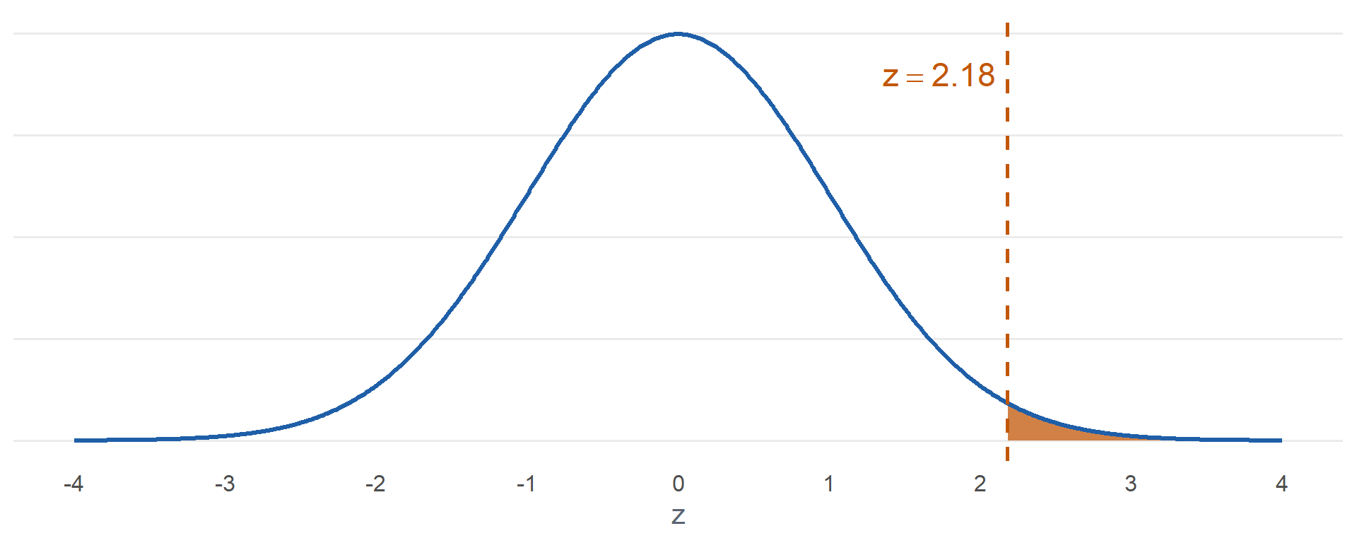
\[z = \frac{0.8400 - 0.7357}{\sqrt{0.7897(0.2103)\left(\dfrac{1}{150}+\dfrac{1}{140}\right)}} = \frac{0.1043}{0.0479} = \mathbf{2.18}\]
4. P-value: Find it.
TipAnswer
\[P(Z \ge 2.18) = \mathbf{0.0147}\]
1 - pnorm(2.178)
5. Decision: Reject or fail to reject?
TipAnswer
\(0.0147 \le 0.05\). Reject \(H_0\).
6. Conclusion: State it in context.
TipAnswer
Since the P-value \(0.0147 \le \alpha = 0.05\), reject \(H_0\). At the 5% level there is sufficient evidence that the true proportion of cadets who finish the 12 mile ruck in 3 hours or less is higher in new boots than in old boots.
Confidence interval: Build a 95% interval for \(p_1 - p_2\) and interpret it.
TipAnswer
Not pooled: each group keeps its own \(\hat{p}_i\).
\[\text{SE} = \sqrt{\frac{0.8400(0.1600)}{150}+\frac{0.7357(0.2643)}{140}} = 0.0478\]
\[0.1043 \pm 1.96(0.0478) = (0.011,\ 0.198)\]
We are 95% confident that the true pass rate in new boots is between 1.1 and 19.8 percentage points higher than in old boots. All positive, consistent with rejecting \(H_0\).
In R
    2-sample test for equality of proportions without continuity correction

data:  c(126, 103) out of c(150, 140)
X-squared = 4.7413, df = 1, p-value = 0.01472
alternative hypothesis: greater
95 percent confidence interval:
 0.02566157 1.00000000
sample estimates:
   prop 1    prop 2
0.8400000 0.7357143 x= successes,n= sample sizes, group 1 firstcorrect = FALSEmatches the \(z\) test by handX-squaredis \(z^2\): \(2.18^2 = 4.741\). Same P-value.- One-sided
alternative, so R prints a one-sided bound, not the two-sided interval. Usealternative = "two.sided"(or compute by hand) for the two-sided interval.
Inference Procedures
| Parameter | Conditions | Test statistic | Confidence interval | Critical value | P-value by \(H_a\) |
|---|---|---|---|---|---|
| \(\mu\) \(\sigma\) known, or \(\sigma\) unknown and \(n > 40\) |
Random sample \(\sigma\) known and population normal, or \(n > 40\) |
\(z = \dfrac{\bar{x} - \mu_0}{\sigma/\sqrt{n}}\) use \(s\) for \(\sigma\) when \(n > 40\) |
\(\bar{x} \pm z_{\alpha/2}\dfrac{\sigma}{\sqrt{n}}\) | qnorm(1-a/2) |
\(>\) 1-pnorm(z)\(<\) pnorm(z)\(\ne\) 2*pnorm(-abs(z)) |
| \(\mu\) \(\sigma\) unknown, \(n \le 40\) |
Random sample Population approx. normal |
\(t = \dfrac{\bar{x} - \mu_0}{s/\sqrt{n}} \sim t_{n-1}\) | \(\bar{x} \pm t_{\alpha/2,\,n-1}\dfrac{s}{\sqrt{n}}\) | qt(1-a/2,n-1) |
\(>\) 1-pt(t,n-1)\(<\) pt(t,n-1)\(\ne\) 2*pt(-abs(t),n-1) |
| \(p\) | Random sample \(np_0 \ge 10\) \(n(1-p_0) \ge 10\) |
\(z = \dfrac{\hat{p} - p_0}{\sqrt{p_0(1-p_0)/n}}\) the test uses \(p_0\) |
\(\hat{p} \pm z_{\alpha/2}\sqrt{\dfrac{\hat{p}(1-\hat{p})}{n}}\) the interval uses \(\hat{p}\) |
qnorm(1-a/2) |
\(>\) 1-pnorm(z)\(<\) pnorm(z)\(\ne\) 2*pnorm(-abs(z)) |
| \(\mu_1 - \mu_2\) independent |
Two independent samples Both normal, or both \(n > 40\) |
\(t = \dfrac{(\bar{x}_1 - \bar{x}_2) - \Delta_0}{\sqrt{s_1^2/n_1 + s_2^2/n_2}} \sim t_{\nu}\) | \((\bar{x}_1 - \bar{x}_2) \pm t_{\alpha/2,\,\nu}\sqrt{\dfrac{s_1^2}{n_1}+\dfrac{s_2^2}{n_2}}\) | qt(1-a/2,nu) |
\(>\) 1-pt(t,nu)\(<\) pt(t,nu)\(\ne\) 2*pt(-abs(t),nu) |
| \(\mu_D\) paired |
Random sample of pairs Differences approx. normal, or \(n > 40\) |
\(t = \dfrac{\bar{d} - \Delta_0}{s_D/\sqrt{n}} \sim t_{n-1}\) | \(\bar{d} \pm t_{\alpha/2,\,n-1}\dfrac{s_D}{\sqrt{n}}\) | qt(1-a/2,n-1) |
\(>\) 1-pt(t,n-1)\(<\) pt(t,n-1)\(\ne\) 2*pt(-abs(t),n-1) |
| \(p_1 - p_2\) | Two independent samples \(n_i\hat{p}_i \ge 10\) \(n_i(1-\hat{p}_i) \ge 10\) |
\(z = \dfrac{\hat{p}_1 - \hat{p}_2}{\sqrt{\hat{p}(1-\hat{p})\left(\frac{1}{n_1}+\frac{1}{n_2}\right)}}\) pooled \(\hat{p} = \dfrac{x_1+x_2}{n_1+n_2}\) |
\((\hat{p}_1 - \hat{p}_2) \pm z_{\alpha/2}\sqrt{\dfrac{\hat{p}_1(1-\hat{p}_1)}{n_1}+\dfrac{\hat{p}_2(1-\hat{p}_2)}{n_2}}\) not pooled |
qnorm(1-a/2) |
\(>\) 1-pnorm(z)\(<\) pnorm(z)\(\ne\) 2*pnorm(-abs(z)) |
Board Problems
Problem 1: Name the Test
NoteQuestions
Choose from: \(z\) test for a mean, one-sample \(t\), one-proportion \(z\), two-sample \(t\), paired \(t\), two-proportion \(z\).
Do fewer than 30% of cadets drink coffee daily? \(250\) cadets surveyed.
Is the proportion of cadets who pass the swim test on the first attempt different for recruited athletes and non-athletes? \(120\) of each.
\(18\) cadets take a reaction time test once rested and once after a 24 hour field exercise.
Mean GPA of \(25\) cadets from each of two regiments.
Mean push-up count of \(60\) cadets compared to the standard of \(50\).
TipAnswers
One-proportion \(z\). One group, yes/no, compared to \(0.30\).
Two-proportion \(z\). Two independent groups, yes/no.
Paired \(t\). Same cadets twice.
Two-sample \(t\). Two independent groups, a numeric outcome.
\(z\) test for a mean. One group, \(n > 40\), use \(s\) for \(\sigma\).
Problem 2: Air Assault
Cadets who attended an optional prep course and cadets who did not were each randomly sampled from those who started Air Assault School. Is the graduation rate different? Test at \(\alpha = 0.10\).
| Group | Started | Graduated |
|---|---|---|
| 1: Prep course | 60 | 41 |
| 2: No prep | 58 | 30 |
NoteQuestions
State the hypotheses.
Check the conditions.
Compute \(\hat{p}_1\), \(\hat{p}_2\), the pooled \(\hat{p}\), and \(z\).
Find the P-value.
Decide and conclude.
Build and interpret a 90% interval for \(p_1 - p_2\).
TipAnswers
- \[H_0: p_1 - p_2 = 0\]
\[H_a: p_1 - p_2 \ne 0\]
\(p_1\) and \(p_2\) are the true graduation rates of cadets with and without the prep course.
Two independent random samples. \(41\), \(19\), \(30\), \(28\) all \(\ge 10\).
\[\hat{p}_1 = \frac{41}{60} = 0.6833, \qquad \hat{p}_2 = \frac{30}{58} = 0.5172, \qquad \hat{p} = \frac{71}{118} = 0.6017\]
\[z = \frac{\hat{p}_1 - \hat{p}_2}{\sqrt{\hat{p}(1-\hat{p})\left(\dfrac{1}{n_1}+\dfrac{1}{n_2}\right)}}\]
\[z = \frac{0.6833 - 0.5172}{\sqrt{0.6017(0.3983)\left(\frac{1}{60}+\frac{1}{58}\right)}} = \frac{0.1661}{\sqrt{0.6017(0.3983)\left(\frac{1}{60}+\frac{1}{58}\right)}} = \frac{0.1661}{0.0901} = \mathbf{1.84}\]
- \[2P(Z \ge 1.84) = \mathbf{0.0654}\]
2 * pnorm(-abs(1.843))
Since the P-value \(0.0654 \le \alpha = 0.10\), reject \(H_0\). At the 10% level there is sufficient evidence that the true Air Assault graduation rate differs between cadets with and without the prep course.
\(z_{0.05} = 1.645\).
qnorm(0.95)
\[0.1661 \pm 1.645(0.0889) = (0.020,\ 0.312)\]
We are 90% confident that the true graduation rate with the prep course is between 2 and 31.2 percentage points higher than without it. All positive, consistent with rejecting at \(\alpha = 0.10\).
Problem 3: Read the Output
During Cadet Basic Training, one company’s barracks had new air filters and another’s did not. A cadet counts as a sick call if they went to sick call at least once. Group 1 is the filtered barracks.
    2-sample test for equality of proportions without continuity correction

data:  c(18, 31) out of c(220, 230)
X-squared = 3.2508, df = 1, p-value = 0.03569
alternative hypothesis: less
95 percent confidence interval:
 -1.000000000 -0.005051453
sample estimates:
    prop 1     prop 2
0.08181818 0.13478261
NoteQuestions
What are \(H_0\) and \(H_a\)? What claim is being tested?
Report \(\hat{p}_1\), \(\hat{p}_2\), \(z\), and the P-value.
Decide at \(\alpha = 0.05\) and conclude in context.
Is the printed interval the two-sided 95% interval for \(p_1 - p_2\)? Why or why not?
TipAnswers
\(H_0: p_1 - p_2 = 0\) versus \(H_a: p_1 - p_2 < 0\), from “alternative hypothesis: less.” The claim: the filtered barracks has a lower sick call rate.
\(\hat{p}_1 = 0.0818\), \(\hat{p}_2 = 0.1348\). \(z = -\sqrt{3.2508} = -1.80\), negative because \(\hat{p}_1 < \hat{p}_2\). P-value \(= 0.0357\).
\(0.0357 \le 0.05\). Reject \(H_0\). At the 5% level there is sufficient evidence that the true proportion of cadets who go to sick call is lower in barracks with new air filters.
No. A one-sided test prints a one-sided bound, here \((-1, -0.0051)\). The two-sided interval is \((-0.110,\ 0.004)\).
Problem 4: Sapper Leader Course
From one company, \(9\) of \(12\) cadets who attended Sapper Leader Course graduated. From another, \(6\) of \(10\) graduated. A classmate wants to run a two-proportion \(z\) test.
NoteQuestions
Check the conditions.
Can we use the two-proportion \(z\) test here?
TipAnswers
\(n_1\hat{p}_1 = 9\), \(n_1(1-\hat{p}_1) = 3\), \(n_2\hat{p}_2 = 6\), \(n_2(1-\hat{p}_2) = 4\). None reach \(10\).
No. The samples are too small for the normal approximation, so the \(z\) P-value is not trustworthy. We would need more cadets in each group.
Before You Leave
Today
- Two independent groups, yes/no outcome: compare \(p_1 - p_2\)
- \(z = \dfrac{\hat{p}_1 - \hat{p}_2}{\sqrt{\hat{p}(1-\hat{p})\left(\frac{1}{n_1}+\frac{1}{n_2}\right)}}\), pooled \(\hat{p} = \dfrac{x_1+x_2}{n_1+n_2}\)
- Interval: \((\hat{p}_1 - \hat{p}_2) \pm z_{\alpha/2}\sqrt{\dfrac{\hat{p}_1(1-\hat{p}_1)}{n_1}+\dfrac{\hat{p}_2(1-\hat{p}_2)}{n_2}}\)
- The test pools, the interval does not
prop.test(x = c(x1, x2), n = c(n1, n2), alternative = "greater", correct = FALSE)
Any questions?
Next Lesson
- Review Lessons 18-26
Upcoming Graded Events
- WebAssign 9.4: due at the start of Lesson 27
- WPR II: Lesson 28 (covers Lessons 18-26)
- TEE: 15-18 Dec 2026