Lesson 30: Simple Linear Regression II
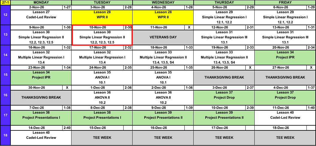
Calendar
Admin
- Project partners: Select your project partner
- Partner status (as of 9 Nov): 13 of 51 cadets still need a partner (B2: 5, C2: 8, D2: 0)
- Project: we talk about it at the end of class
What We Did: Lesson 29
NoteKey Concepts from Lesson 29
- Model: \(Y = \beta_0 + \beta_1 x + \varepsilon\), \(\varepsilon \sim N(0, \sigma^2)\)
- Least squares: choose \(\hat{\beta}_0\), \(\hat{\beta}_1\) to minimize \(\sum (y_i - \hat{y}_i)^2\)
- \(\hat{\beta}_1 = \dfrac{\sum (x_i - \bar{x})(y_i - \bar{y})}{\sum (x_i - \bar{x})^2}\), \(\hat{\beta}_0 = \bar{y} - \hat{\beta}_1\bar{x}\)
- Slope: change in the mean of \(y\) for a one unit increase in \(x\)
- Predict only inside the range of the \(x\) data
NoteReview: Statistical Inference (Lessons 18 to 26)
- Confidence interval: \(\text{estimate} \pm \text{critical value} \times \text{standard error}\)
- Six steps: hypotheses, conditions, test statistic, P-value, decision, conclusion
- One group: \(z\) or \(t\) for \(\mu\), \(z\) for \(p\)
- Two groups: two-sample \(t\) for \(\mu_1 - \mu_2\), paired \(t\) for \(\mu_D\), two-proportion \(z\) for \(p_1 - p_2\)
What We’re Doing: Lesson 30
Objectives
- Carry out a \(t\) test for the slope \(\beta_1\). (SLO 5)
- Compute and interpret the coefficient of determination \(r^2\) (from SSE and SST). (SLO 2, 4)
- Fit a simple linear regression in R and interpret the standard software output: estimated coefficients, standard errors, \(t\) statistics and \(P\)-values, and \(r^2\). (SLO 4)
Required Reading
Devore 12.2, 12.3, 12.5
Break!
DMath Intramurals
DMath Frisbee!!

Math vs CBSE
NoteResult
10-0
15-12
DMath Basketball!!

Game 1
NoteResult
1-0
Math vs DPW
NoteResult
1-1
DMath Volleyball!!

Math vs DPE
NoteResult
0-1
The Takeaway for Today
NoteKey Concepts from Lesson 30
- Least squares: \(\hat{\beta}_1 = \dfrac{\sum (x_i - \bar{x})(y_i - \bar{y})}{\sum (x_i - \bar{x})^2}\), \(\hat{\beta}_0 = \bar{y} - \hat{\beta}_1\bar{x}\)
- Slope test: \(H_0: \beta_1 = 0\), \(t = \hat{\beta}_1 / s_{\hat{\beta}_1}\), df \(= n - 2\)
- \(r^2 = 1 - \text{SSE}/\text{SST}\): proportion of variation in \(y\) explained by the line
Lesson 29, Again
Same ruck data, start to finish. Then we build on it.
The Data
Does pack weight slow cadets down? Twelve cadets each rucked 12 miles with a different pack weight.
| Cadet | 1 | 2 | 3 | 4 | 5 | 6 | 7 | 8 | 9 | 10 | 11 | 12 |
|---|---|---|---|---|---|---|---|---|---|---|---|---|
| Weight \(x\) (lb) | 25 | 28 | 30 | 33 | 35 | 38 | 40 | 44 | 47 | 50 | 55 | 60 |
| Time \(y\) (min) | 156 | 159 | 168 | 174 | 166 | 185 | 173 | 175 | 184 | 191 | 192 | 204 |
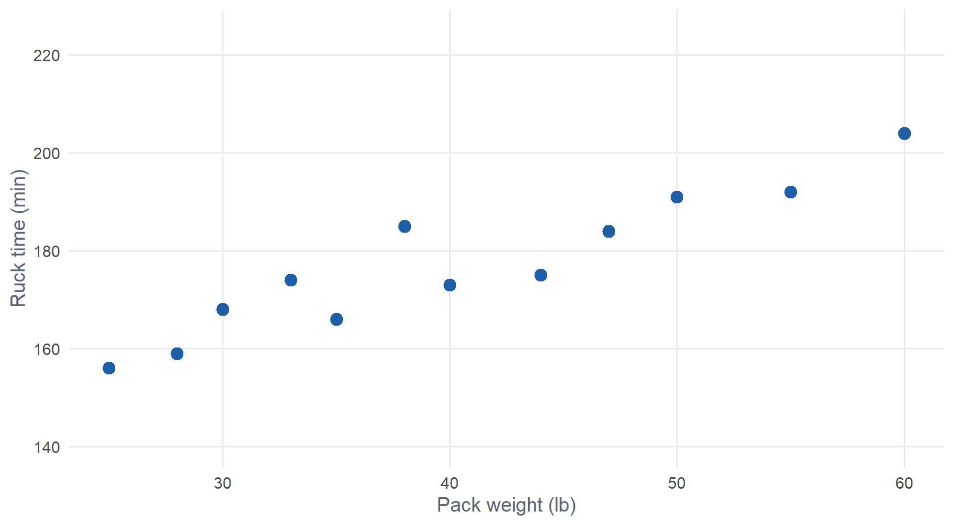
- Response \(y\): ruck time. Explanatory \(x\): pack weight.
- Direction: positive. Form: roughly linear. Strength: fairly strong. Unusual observations: none.
Which Line Is Best?
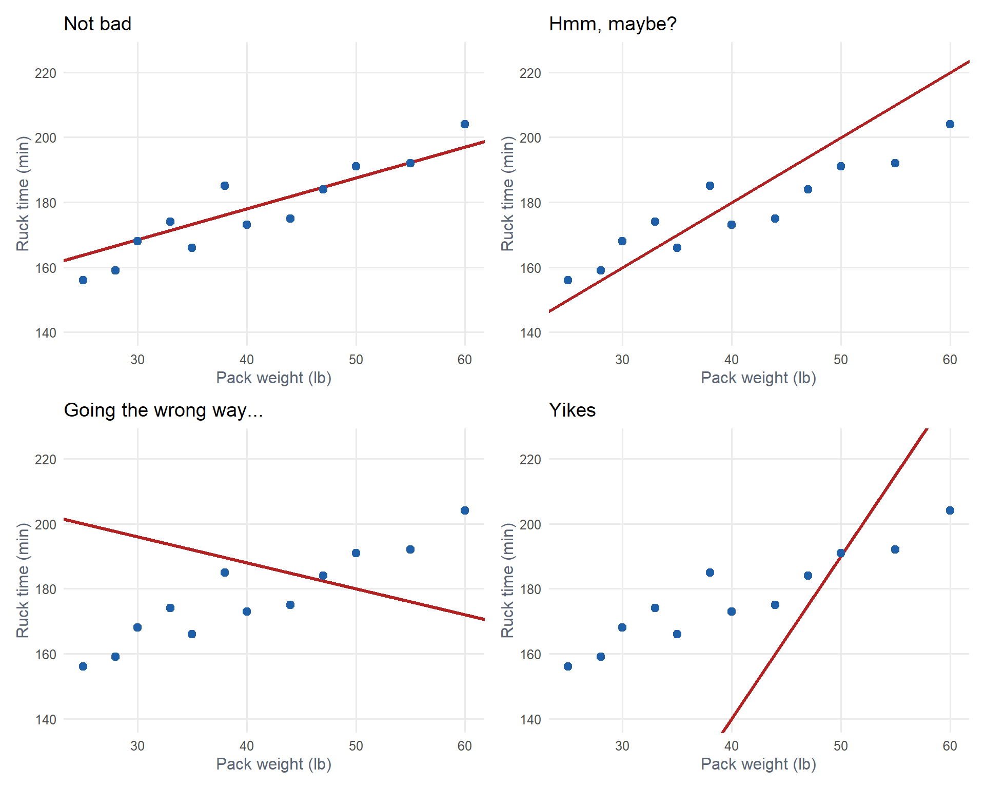
We want the line that minimizes the grey lines.
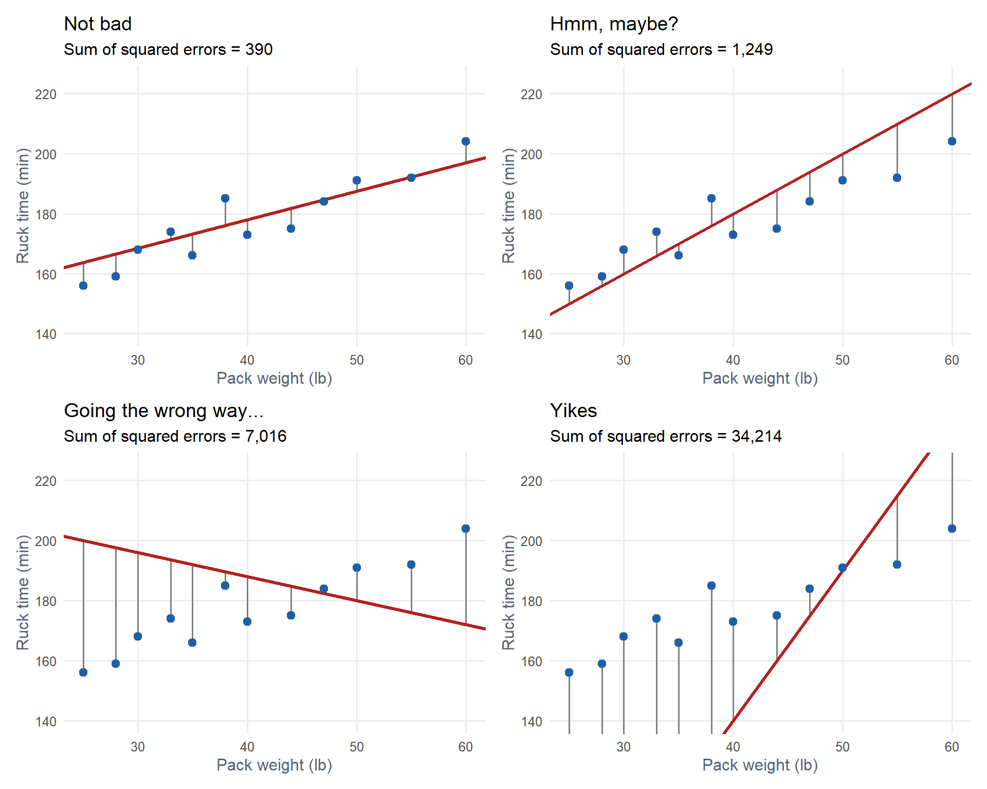
Each line is written
\[\hat{y} = \hat{\beta}_0 + \hat{\beta}_1 x\]
Each grey segment is an error (residual): \(e_i = y_i - \hat{y}_i\).
The least squares line chooses \(\hat{\beta}_0\) and \(\hat{\beta}_1\) to minimize
\[\text{SSE} = \sum_{i=1}^{n} (y_i - \hat{y}_i)^2 = \sum_{i=1}^{n} \left(y_i - \hat{\beta}_0 - \hat{\beta}_1 x_i\right)^2\]
ImportantLeast Squares Estimates
\[\hat{\beta}_1 = \frac{\sum (x_i - \bar{x})(y_i - \bar{y})}{\sum (x_i - \bar{x})^2}, \qquad \hat{\beta}_0 = \bar{y} - \hat{\beta}_1 \bar{x}\]
Ruck data: \(\bar{x} = 40.42\), \(\bar{y} = 177.25\), \(\sum (x_i - \bar{x})(y_i - \bar{y}) = 1625.75\), \(\sum (x_i - \bar{x})^2 = 1334.92\)
\[\hat{\beta}_1 = \frac{1625.75}{1334.92} = 1.2179, \qquad \hat{\beta}_0 = 177.25 - 1.2179(40.42) = 128.03\]
The Model
ImportantSimple Linear Regression Model
\[Y = \beta_0 + \beta_1 x + \varepsilon, \qquad \varepsilon \sim N(0, \sigma^2)\]
- \(\beta_0\), \(\beta_1\): true intercept and slope, parameters. \(\hat{\beta}_0\), \(\hat{\beta}_1\): their least squares estimates.
- True regression line: \(\mu_{Y \cdot x} = \beta_0 + \beta_1 x\), the mean of \(Y\) at a given \(x\)
- Linear: the mean of \(Y\) is a straight line in \(x\)
- Independent: the errors \(\varepsilon_i\) are independent
- Normal: the errors are normally distributed
- Equal variance: \(\sigma^2\) is the same at every \(x\)
Fitting It in R
ruck <- data.frame(
  weight = c(25, 28, 30, 33, 35, 38, 40, 44, 47, 50, 55, 60),
  time   = c(156, 159, 168, 174, 166, 185, 173, 175, 184, 191, 192, 204)
)
model <- lm(time ~ weight, data = ruck)
summary(model)
Call:
lm(formula = time ~ weight, data = ruck)

Residuals:
   Min     1Q Median     3Q    Max
-6.614 -3.282 -1.871  3.034 10.693

Coefficients:
            Estimate Std. Error t value Pr(>|t|)
(Intercept) 128.0279     6.0311  21.228 1.20e-09 ***
weight        1.2179     0.1444   8.435 7.39e-06 ***
---
Signif. codes:  0 '***' 0.001 '**' 0.01 '*' 0.05 '.' 0.1 ' ' 1

Residual standard error: 5.275 on 10 degrees of freedom
Multiple R-squared:  0.8768,    Adjusted R-squared:  0.8644
F-statistic: 71.14 on 1 and 10 DF,  p-value: 7.386e-06
The Regression Equation
Read the Estimate column: (Intercept) is \(\hat{\beta}_0\), weight is \(\hat{\beta}_1\).
\[\widehat{\text{time}} = 128.03 + 1.22\,(\text{weight})\]
ImportantInterpreting Slope and Intercept
Slope (\(\hat{\beta}_1 = 1.22\)): for each additional pound of pack weight, the estimated mean 12 mile ruck time increases by 1.22 minutes.
Intercept (\(\hat{\beta}_0 = 128.03\)): the estimated mean ruck time with a 0 lb pack. Not meaningful: 0 lb is outside the data (25 to 60 lb).
WarningContext Matters
- Interpret the slope with units and context. “The slope is 1.22” is not enough.
- If \(x = 0\) is outside the data, the intercept may not be meaningful. Say so.
The P-Values: Hypothesis Tests
There is a P-value at the end of each row. Where there’s a P-value, there’s a hypothesis test.
             Estimate Std. Error t value  Pr(>|t|)
(Intercept) 128.02790    6.03114 21.2278 1.198e-09 ***
weight        1.21787    0.14439  8.4346 7.386e-06 ***
NoteHypothesis Tests in the Output
Slope: is there a linear relationship between \(x\) and \(y\)?
\[H_0: \beta_1 = 0 \qquad H_a: \beta_1 \neq 0\]
If \(\beta_1 = 0\), the true line is flat: \(x\) tells us nothing about the mean of \(Y\). This is the test we care about.
Intercept: is the true intercept different from zero?
\[H_0: \beta_0 = 0 \qquad H_a: \beta_0 \neq 0\]
Usually not of interest.
Important\(t\) Test for the Slope
\[T = \frac{\hat{\beta}_1 - 0}{s_{\hat{\beta}_1}} \sim t_{n-2}\]
- \(\hat{\beta}_1\):
Estimate. \(s_{\hat{\beta}_1}\):Std. Error. \(T\):t value. P-value: Pr(>|t|). - By hand: \(s = \sqrt{\dfrac{\text{SSE}}{n - 2}}\) (R’s
Residual standard error), \(s_{\hat{\beta}_1} = \dfrac{s}{\sqrt{\sum (x_i - \bar{x})^2}}\)
Ruck Weight
Is there a linear relationship between pack weight and ruck time? Use \(\alpha = 0.05\).
\[H_0: \beta_1 = 0\]
\[H_a: \beta_1 \neq 0\]
Test statistic. From the weight row:
\[t = \frac{\hat{\beta}_1 - 0}{s_{\hat{\beta}_1}}\]
\[t = \frac{1.2179}{0.1444} = 8.43\]
P-value. df \(= 10\). P-value \(= 2P(T > 8.43) = 7.39 \times 10^{-6}\)
2 * (1 - pt(8.435, 10))
Decision and conclusion. P-value \(\le 0.05\), so reject \(H_0\). There is convincing evidence of a linear relationship between pack weight and 12 mile ruck time.
Intercept row: \(t = 21.23\), P-value \(= 1.20 \times 10^{-9}\). Reject \(H_0: \beta_0 = 0\), but we don’t care: 0 lb is outside the data.
Making Predictions
How long would we expect a cadet carrying 45 lb to take on the 12 mile ruck?
\[\widehat{\text{time}} = 128.03 + 1.22(45) = \mathbf{182.83} \text{ minutes}\]
predict(model, newdata = data.frame(weight = 45)) 1
182.8319
WarningInterpolation vs. Extrapolation
- Interpolation: predicting inside the observed \(x\) range (25 to 60 lb). Fine.
- Extrapolation: predicting outside it. The line may not continue.
- 45 lb is interpolation. 100 lb would be extrapolation.
How Good Is the Fit? \(r^2\)
ImportantCoefficient of Determination
\[r^2 = 1 - \frac{\text{SSE}}{\text{SST}}, \qquad \text{SST} = \sum (y_i - \bar{y})^2, \qquad \text{SSE} = \sum (y_i - \hat{y}_i)^2\]
Ruck data: Multiple R-squared \(= 0.8768\). About 87.7% of the variation in ruck time is explained by pack weight.
The Project
The question: answer a real question for a real Army decision maker, using real unit data in Vantage.
What Your Analysis Needs
- A research question you and your partner developed, for a named decision maker
- A one-sample test: compare your unit to a standard or benchmark. One-sample \(t\), or one-proportion \(z\) for categorical data.
- A two-sample test: compare two groups in your unit. Two-sample \(t\), or two-proportion \(z\) for categorical data.
- A regression (required):
lm(response ~ proxy). Slope test, \(r^2\). Check LINE (Lesson 31), then add predictors (Lessons 32, 33). - Every test: hypotheses, test statistic, P-value, decision and conclusion in context
Graded Events
| Event | When | What | Points |
|---|---|---|---|
| EDA | Lesson 14 | Research question, decision maker, construct, proxy, initial EDA | 25 |
| IPR | Lesson 34 (20, 23 Nov) | Your project as finished as possible. Instructor and peer feedback. | 25 |
| Products | Lesson 37 (3, 4 Dec) | Slide deck, executive summary, analysis code in Canvas | 50 |
| Brief | Lessons 38, 39 (7 to 10 Dec) | 5 minute BLUF brief, 10 minute defense led by your instructor | 100 |
The IPR: come in as close to done as you can. A finished draft gets feedback you can use. A plan gets “go do the analysis.”
This Week
- Pick a partner: Select your project partner. As of 9 Nov, 13 cadets still need one.
- Settle the research question with your partner.
- Run the one-sample and two-sample tests in Vantage now. You already know how.
The Brief
- BLUF first: answer the decision maker’s question in one sentence.
- Every number gets an interpretation in context.
- Defense: expect “Why this proxy?”, “Do the assumptions hold?”, “What would change your answer?”
AI: Level 2. Use it and document it IAW the DAAW. You own every number you brief.
Let’s Go to Vantage!
# MA206 Exploratory Data Analysis: Brigade Readiness

library(tidyverse)
library(foundry)

# Read the full AY27-1 readiness dataset from Foundry.
master <- datasets.read_table("ay27_1_master")

# Select the brigade used in the EDA report.
MY_BRIGADE <- "20TH ENGINEER BRIGADE"
bde <- master |>
  filter(BrigadeName == MY_BRIGADE) |>
  select(age, time_in_active_service_years, skill_level, height, weight, aft_score_total) |>
  filter(!is.na(aft_score_total))

# Create model
mod <- lm(weight~height, data = bde)
summary(mod)- Is height a useful linear predictor of weight? Which row, which number?
- What proportion of the variation in weight is explained by height?
Before You Leave
Today
- Least squares line: \(\hat{\beta}_1 = \dfrac{\sum (x_i - \bar{x})(y_i - \bar{y})}{\sum (x_i - \bar{x})^2}\), \(\hat{\beta}_0 = \bar{y} - \hat{\beta}_1\bar{x}\)
- \(s = \sqrt{\text{SSE}/(n-2)}\), \(s_{\hat{\beta}_1} = s / \sqrt{\sum (x_i - \bar{x})^2}\)
- Slope test: \(t = \hat{\beta}_1 / s_{\hat{\beta}_1}\), df \(= n - 2\)
- \(r^2 = 1 - \text{SSE}/\text{SST}\)
Any questions?
Next Lesson
Lesson 31: Simple Linear Regression III
- 12, 13 Nov
- Devore 13.1
- Residual plots and normal probability plots
- Checking the LINE assumptions
Upcoming Graded Events
- WebAssign 12.2, 12.3, 12.5: due at the start of Lesson 31
- Project IPR: Lesson 34 (20, 23 Nov)
- TEE: 15 to 18 Dec 2026