Lesson 27: Cadet-Led Review

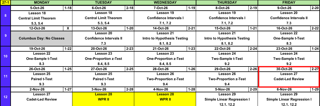
Calendar

WPR II Admin

WPR II: Lesson 28 (3, 4 Nov)

Covers: Lessons 18 through 26
Time: 55 minutes
Authorized: the course statistics reference card (SRC), R-Lite, and the issued calculator

R-Lite and the SRC

Have R-Lite working and know your SRC before you walk in

Download R-Lite from Canvas.
Open it and run one call, like pt(2, 10), today.
Not working? Tell me today, not at the start of the WPR.
Open the SRC and know where every formula and table lives.

Study Materials

WPR II Review and Key on Canvas

What We’re Doing: Lesson 27

Objectives

Review Lessons 18-26.

Required Reading

None

Break!

Cadet-Led Review

Block II Outline

Sampling Distributions and Confidence Intervals

Lesson 18: Central Limit Theorem (Devore 5.3, 5.4)

Statistic varies sample to sample, its distribution is the sampling distribution
\(\bar{X} \sim N\left(\mu,\ \left(\dfrac{\sigma}{\sqrt{n}}\right)^2\right)\), approximately, for \(n > 40\)
Normal population: exact for any \(n\)
Standard error \(\sigma/\sqrt{n}\) shrinks as \(n\) grows
pnorm(x, mu, sigma/sqrt(n))
\(\hat{p} \sim N\left(p,\ \dfrac{p(1-p)}{n}\right)\), approximately, when \(np \ge 10\) and \(n(1-p) \ge 10\)

Lesson 19: Confidence Intervals I (Devore 7.1, 7.2)

\(\text{estimate} \pm \text{critical value} \times \text{standard error}\)
Mean, \(n > 40\): \(\bar{x} \pm z_{\alpha/2}\,\dfrac{s}{\sqrt{n}}\)
Proportion, \(n\hat{p} \ge 10\) and \(n(1-\hat{p}) \ge 10\): \(\hat{p} \pm z_{\alpha/2}\sqrt{\dfrac{\hat{p}(1-\hat{p})}{n}}\)
qnorm(0.975) for 95%, qnorm(0.95) for 90%, qnorm(0.995) for 99%
95% confident describes the method, not one interval

Lesson 20: Confidence Intervals II (Devore 7.3)

Small sample, normal population: \(\bar{x} \pm t_{\alpha/2,\,n-1}\,\dfrac{s}{\sqrt{n}}\)
\(\text{df} = n - 1\), qt(0.975, n - 1) for 95%
\(t_{\alpha/2,\,n-1} > z_{\alpha/2}\), so the \(t\) interval is wider
Sample size for width \(w\): \(n = \left(\dfrac{2\,z_{\alpha/2}\,\sigma}{w}\right)^2\), rounded up

Hypothesis Tests

Lesson 21: Intro to Hypothesis Testing (Devore 8.1, 8.2)

\(H_0\) has the \(=\), the claim goes in \(H_a\): \(<\), \(>\), or \(\ne\)
\(z = \dfrac{\bar{x} - \mu_0}{s/\sqrt{n}}\), random sample, \(n > 40\)
P-value: probability of a result at least this extreme if \(H_0\) is true
Reject \(H_0\) if the P-value is at or below \(\alpha\), otherwise fail to reject
Type I: reject a true \(H_0\) (\(\alpha\)). Type II: fail to reject a false \(H_0\) (\(\beta\))
Fail to reject is not accept

Lesson 22: One-Sample t-Test (Devore 8.3)

\(t = \dfrac{\bar{x} - \mu_0}{s/\sqrt{n}}\), \(\text{df} = n - 1\)
Random sample, \(n \le 40\), population approximately normal
P-value: pt(t, n - 1), 1 - pt(t, n - 1), 2 * pt(-abs(t), n - 1)
t.test(x, mu = mu0, alternative = "two.sided")

Lesson 23: One-Proportion z-Test (Devore 8.4, 8.5)

\(z = \dfrac{\hat{p} - p_0}{\sqrt{p_0(1 - p_0)/n}}\)
Random sample, \(np_0 \ge 10\) and \(n(1 - p_0) \ge 10\)
The test uses \(p_0\), the interval uses \(\hat{p}\)
Statistically significant does not mean practically significant

Lesson 24: Two-Sample t-Test (Devore 9.2)

\(t = \dfrac{(\bar{x}_1 - \bar{x}_2) - \Delta_0}{\sqrt{s_1^2/n_1 + s_2^2/n_2}}\), approximate df \(\nu\), rounded down
Two independent random samples, both populations approximately normal (or both \(n > 40\))
Interval: \((\bar{x}_1 - \bar{x}_2) \pm t_{\alpha/2,\,\nu}\sqrt{s_1^2/n_1 + s_2^2/n_2}\)
Name group 1 first, then put the claim in \(H_a\)
t.test(x1, x2, alternative = "greater")

Lesson 25: Paired t-Test (Devore 9.3)

Paired data: two measurements on the same unit. Analyze the differences \(d_i\).
\(t = \dfrac{\bar{d} - \Delta_0}{s_D/\sqrt{n}}\), \(\text{df} = n - 1\), a one-sample \(t\) on the differences
Interval: \(\bar{d} \pm t_{\alpha/2,\,n-1}\dfrac{s_D}{\sqrt{n}}\)
Pairing removes unit to unit variability, so the standard error shrinks
t.test(x, y, paired = TRUE, alternative = "greater")

Lesson 26: Two-Proportion z-Test (Devore 9.4)

Two independent groups, a yes/no outcome: compare \(p_1 - p_2\)
\(z = \dfrac{\hat{p}_1 - \hat{p}_2}{\sqrt{\hat{p}(1-\hat{p})\left(\frac{1}{n_1}+\frac{1}{n_2}\right)}}\), pooled \(\hat{p} = \dfrac{x_1+x_2}{n_1+n_2}\)
Conditions: \(n_i\hat{p}_i \ge 10\) and \(n_i(1-\hat{p}_i) \ge 10\) in both groups
The test pools, the interval does not

The Six Steps

Hypotheses: \(H_0\) and \(H_a\), and define the parameter in context
Conditions: name them and check them with the numbers
Test statistic: formula first, then plug in
P-value: direction from \(H_a\), R-Lite call
Decision: compare the P-value to \(\alpha\), reject or fail to reject \(H_0\)
Conclusion: at the \(\alpha\) level, sufficient (or insufficient) evidence that \(H_a\), in context

Which Test?

flowchart TD
  A{"Mean or<br>proportion?"} -->|"Mean"| M{"One group or two?"}
  A -->|"Proportion"| P{"One group or two?"}
  M -->|"One"| S{"Small or large<br>sample?"}
  M -->|"Two"| D{"Paired or<br>independent?"}
  P -->|"Two"| P2["Two-proportion z<br>p1 - p2"]
  P -->|"One"| P1["One-proportion z<br>p"]
  S -->|"Large: n > 40,<br>or σ known"| Z["z for a mean<br>μ"]
  S -->|"Small: n ≤ 40,<br>σ unknown"| T["One-sample t<br>μ"]
  D -->|"Paired: same units<br>measured twice"| PD["Paired t<br>μD"]
  D -->|"Independent:<br>different units"| I["Two-sample t<br>μ1 - μ2"]

Inference Procedures

Parameter	Conditions	Test statistic	Confidence interval	Critical value	P-value by \(H_a\)
\(\mu\) \(\sigma\) known, or \(\sigma\) unknown and \(n > 40\)	Random sample \(\sigma\) known and population normal, or \(n > 40\)	\(z = \dfrac{\bar{x} - \mu_0}{\sigma/\sqrt{n}}\) use \(s\) for \(\sigma\) when \(n > 40\)	\(\bar{x} \pm z_{\alpha/2}\dfrac{\sigma}{\sqrt{n}}\)	`qnorm(1-a/2)`	\(>\) `1-pnorm(z)` \(<\) `pnorm(z)` \(\ne\) `2*pnorm(-abs(z))`
\(\mu\) \(\sigma\) unknown, \(n \le 40\)	Random sample Population approx. normal	\(t = \dfrac{\bar{x} - \mu_0}{s/\sqrt{n}} \sim t_{n-1}\)	\(\bar{x} \pm t_{\alpha/2,\,n-1}\dfrac{s}{\sqrt{n}}\)	`qt(1-a/2,n-1)`	\(>\) `1-pt(t,n-1)` \(<\) `pt(t,n-1)` \(\ne\) `2*pt(-abs(t),n-1)`
\(p\)	Random sample \(np_0 \ge 10\) \(n(1-p_0) \ge 10\)	\(z = \dfrac{\hat{p} - p_0}{\sqrt{p_0(1-p_0)/n}}\) the test uses \(p_0\)	\(\hat{p} \pm z_{\alpha/2}\sqrt{\dfrac{\hat{p}(1-\hat{p})}{n}}\) the interval uses \(\hat{p}\)	`qnorm(1-a/2)`	\(>\) `1-pnorm(z)` \(<\) `pnorm(z)` \(\ne\) `2*pnorm(-abs(z))`
\(\mu_1 - \mu_2\) independent	Two independent samples Both normal, or both \(n > 40\)	\(t = \dfrac{(\bar{x}_1 - \bar{x}_2) - \Delta_0}{\sqrt{s_1^2/n_1 + s_2^2/n_2}} \sim t_{\nu}\)	\((\bar{x}_1 - \bar{x}_2) \pm t_{\alpha/2,\,\nu}\sqrt{\dfrac{s_1^2}{n_1}+\dfrac{s_2^2}{n_2}}\)	`qt(1-a/2,nu)`	\(>\) `1-pt(t,nu)` \(<\) `pt(t,nu)` \(\ne\) `2*pt(-abs(t),nu)`
\(\mu_D\) paired	Random sample of pairs Differences approx. normal, or \(n > 40\)	\(t = \dfrac{\bar{d} - \Delta_0}{s_D/\sqrt{n}} \sim t_{n-1}\)	\(\bar{d} \pm t_{\alpha/2,\,n-1}\dfrac{s_D}{\sqrt{n}}\)	`qt(1-a/2,n-1)`	\(>\) `1-pt(t,n-1)` \(<\) `pt(t,n-1)` \(\ne\) `2*pt(-abs(t),n-1)`
\(p_1 - p_2\)	Two independent samples \(n_i\hat{p}_i \ge 10\) \(n_i(1-\hat{p}_i) \ge 10\)	\(z = \dfrac{\hat{p}_1 - \hat{p}_2}{\sqrt{\hat{p}(1-\hat{p})\left(\frac{1}{n_1}+\frac{1}{n_2}\right)}}\) pooled \(\hat{p} = \dfrac{x_1+x_2}{n_1+n_2}\)	\((\hat{p}_1 - \hat{p}_2) \pm z_{\alpha/2}\sqrt{\dfrac{\hat{p}_1(1-\hat{p}_1)}{n_1}+\dfrac{\hat{p}_2(1-\hat{p}_2)}{n_2}}\) not pooled	`qnorm(1-a/2)`	\(>\) `1-pnorm(z)` \(<\) `pnorm(z)` \(\ne\) `2*pnorm(-abs(z))`

Problem 1: Shuttle Wait

The time \(X\) (in minutes) a cadet waits for the post shuttle is exponential with mean 6 minutes. A random sample of \(n = 50\) cadets each record one wait. Let \(\bar{X}\) be their sample mean wait.

Questions

\(X\) is skewed right. Why can we still use a normal distribution for \(\bar{X}\)?
Fully specify the distribution of \(\bar{X}\).
Find \(P(\bar{X} > 7)\).
Find the value \(c\) with \(P(\bar{X} > c) = 0.05\).

Answers

CLT. \(n = 50 > 40\), so \(\bar{X}\) is approximately normal whatever the shape of \(X\).
For an exponential, \(\mu = \sigma = 6\) minutes, so

\[\bar{X} \sim N\left(6,\ \left(\frac{6}{\sqrt{50}}\right)^2\right) = N\left(6,\ 0.849^2\right)\]

\(P(\bar{X} > 7) = 1 - P(\bar{X} \le 7) \approx \mathbf{0.119}\) 1 - pnorm(7, 6, 6/sqrt(50))
\(c\) is the 95th percentile of \(\bar{X}\): \(c \approx \mathbf{7.396}\) minutes. qnorm(0.95, 6, 6/sqrt(50))

Problem 2: Name the Test

Questions

Choose from: \(z\) test for a mean, one-sample \(t\), one-proportion \(z\), two-sample \(t\), paired \(t\), two-proportion \(z\).

\(15\) cadets run the 2 mile before and after a six week running program.
Is the proportion of cadets who own a car different in two regiments? \(150\) cadets from each.
Mean nightly sleep of \(64\) cadets compared to \(7\) hours.
Mean ACFT score of \(20\) cadets in one company and \(22\) in another.
Do more than 40% of cadets plan to branch combat arms? \(400\) cadets surveyed.
Mean weight of \(12\) packed rucks compared to \(35\) pounds. Weights are approximately normal.

Answers

Paired \(t\). Same cadets twice.
Two-proportion \(z\). Two independent groups, yes/no.
\(z\) test for a mean. One group, \(n > 40\), use \(s\) for \(\sigma\).
Two-sample \(t\). Two independent groups, a numeric outcome.
One-proportion \(z\). One group, yes/no, compared to \(0.40\).
One-sample \(t\). One group, \(n \le 40\), normal population.

Problem 3: Cadet Sleep

Do cadets average more than 6 hours of sleep a night? A random sample of \(n = 20\) cadets averages \(\bar{x} = 6.5\) hours with \(s = 0.9\) hours. Sleep times are approximately normal. Test at \(\alpha = 0.05\).

Questions

State the hypotheses.
State and check the conditions.
Compute the test statistic.
Find the P-value.
Decide and conclude in context.
Build and interpret a 95% confidence interval for \(\mu\).

Answers

\[H_0: \mu = 6 \qquad H_a: \mu > 6\]

\(\mu\) is the true mean nightly sleep of all cadets, in hours.

One-sample \(t\). Random sample, and \(n = 20 \le 40\), so the population must be approximately normal (given).
\[t = \frac{\bar{x} - \mu_0}{s/\sqrt{n}} = \frac{6.5 - 6}{0.9/\sqrt{20}} = \frac{0.5}{0.2012} = \mathbf{2.48}, \qquad \text{df} = 19\]
\(P(T \ge 2.48) \approx \mathbf{0.011}\) 1 - pt(2.485, 19)
Since the P-value \(0.011 \le \alpha = 0.05\), reject \(H_0\). At the 5% level there is sufficient evidence that the true mean nightly sleep of cadets is more than 6 hours.
\(t_{0.025,\,19} = 2.093\) qt(0.975, 19)

\[6.5 \pm 2.093\left(\frac{0.9}{\sqrt{20}}\right) = 6.5 \pm 0.421 = (6.079,\ 6.921)\]

We are 95% confident that the true mean nightly sleep of cadets is between 6.079 and 6.921 hours.

Problem 4: Left-Handed Cadets

About 10% of adults are left-handed. In a random sample of \(300\) cadets, \(39\) are left-handed. Is the proportion of left-handed cadets different from \(0.10\)? Test at \(\alpha = 0.05\).

Questions

State the hypotheses.
State and check the conditions.
Compute the test statistic.
Find the P-value.
Decide and conclude in context.
Build and interpret a 95% confidence interval for \(p\). Does it agree with your decision?

Answers

\[H_0: p = 0.10 \qquad H_a: p \ne 0.10\]

\(p\) is the true proportion of all cadets who are left-handed.

One-proportion \(z\). Random sample. \(np_0 = 300(0.10) = 30 \ge 10\) and \(n(1 - p_0) = 300(0.90) = 270 \ge 10\).
\(\hat{p} = 39/300 = 0.13\).

\[z = \frac{\hat{p} - p_0}{\sqrt{p_0(1-p_0)/n}} = \frac{0.13 - 0.10}{\sqrt{0.10(0.90)/300}} = \frac{0.03}{0.0173} = \mathbf{1.73}\]

\(2P(Z \ge 1.73) \approx \mathbf{0.083}\) 2 * pnorm(-abs(1.732))
Since the P-value \(0.083 > \alpha = 0.05\), fail to reject \(H_0\). At the 5% level there is insufficient evidence that the true proportion of left-handed cadets differs from 0.10.
The interval uses \(\hat{p}\), not \(p_0\):

\[0.13 \pm 1.96\sqrt{\frac{0.13(0.87)}{300}} = 0.13 \pm 1.96(0.0194) = (0.092,\ 0.168)\]

We are 95% confident that the true proportion of left-handed cadets is between 0.092 and 0.168. It contains \(0.10\), so it agrees with failing to reject.

Before You Leave

Today

Review Lessons 18-26

Any questions?

Next Lesson

Lesson 28: WPR II

Covers Lessons 18-26

Upcoming Graded Events

WPR II: Lesson 28 (covers Lessons 18-26)
TEE: 15-18 Dec 2026