Lesson 13: Generalization

Lesson Administration

Calendar

Day 1

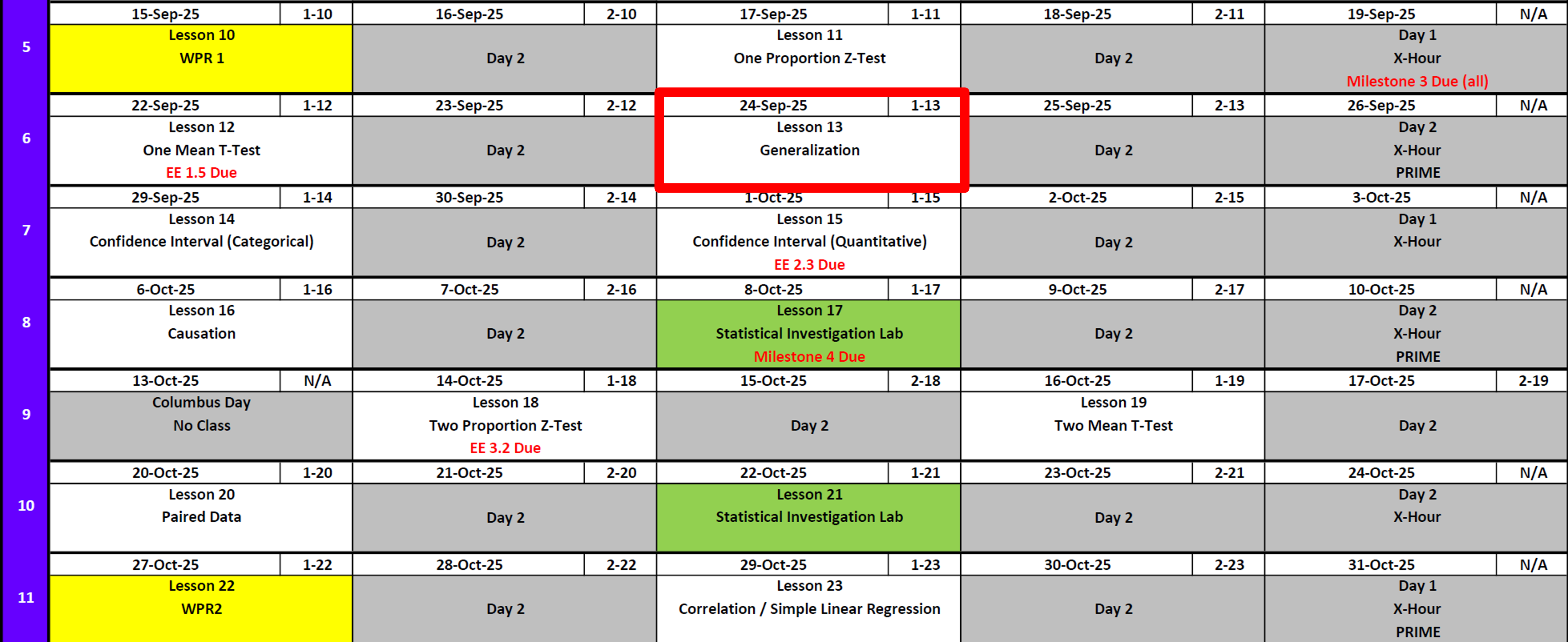
Day 2

Exploration Exercise 1.5

If turned in this morning, can earn 100% of points.
If turned in by 0700 tomorrow morning, can earn 80% of points.

Exploration Exercise 2.3

⏰ Due 0700 ET on 1 October

Milestone 4

Lesson 17
Milestone 4
- With partner
- Write 1-2 paragraphs per article summarizing the articles topic with a take away for its insight on your project.
- Make updates from Milestone 3 feedback.
- Fill out Annex B for my comments on Milestone 3.
- Turn in EVERYTHING in your working write up.
- Keep your binder up-to-date, but I don’t want to see it.

DMath Frisbee Update

Math 1 vs Systems

Previously 3-0

4-0

Reese

Review: \(z\)-Tests for One Proportion

For all cases:

\[ z = \frac{\hat{p} - \pi_0}{\sqrt{\frac{\pi_0 (1 - \pi_0)}{n}}} \]

Alternative Hypothesis	Formula for \(p\)-value	R Code
\(H_A: p > \pi_0\)	\(p = 1 - \Phi(z)\)	`p_val <- 1 - pnorm(z_stat)`
\(H_A: p < \pi_0\)	\(p = \Phi(z)\)	`p_val <- pnorm(z_stat)`
\(H_A: p \neq \pi_0\)	\(p = 2 \cdot (1 - \Phi(\|z\|))\)	`p_val <- 2 * (1 - pnorm(abs(z_stat)))`

Where:

\(\hat{p} = R/n\) (sample proportion)
\(\pi_0\) = hypothesized proportion under \(H_0\)
\(\Phi(\cdot)\) = cumulative distribution function (CDF) of the standard normal distribution.

Review: \(t\)-Tests for One Mean

For all cases:

\[ t = \frac{\bar{x} - \mu_0}{s / \sqrt{n}} \]

Alternative Hypothesis	Formula for \(p\)-value	R Code
\(H_A: \mu > \mu_0\)	\(p = 1 - F_{t_{df}}(t)\)	`p_val <- 1 - pt(t_stat, df)`
\(H_A: \mu < \mu_0\)	\(p = F_{t_{df}}(t)\)	`p_val <- pt(t_stat, df)`
\(H_A: \mu \neq \mu_0\)	\(p = 2 \cdot (1 - F_{t_{df}}(\|t\|))\)	`p_val <- 2 * (1 - pt(abs(t_stat), df))`

Where:

\(\bar{x}\) = sample mean
\(\mu_0\) = hypothesized mean under \(H_0\)
\(s\) = sample standard deviation
\(n\) = sample size
\(df = n - 1\) = degrees of freedom
\(F_{t_{df}}(\cdot)\) = cumulative distribution function (CDF) of the Student’s \(t\) distribution with \(df\) degrees of freedom

Interpreting the \(p\)-value

Rejecting \(H_0\)
> Since the \(p\)-value is less than \(\alpha\) (e.g., \(0.05\)), we reject the null hypothesis.
> We conclude that there is sufficient evidence to suggest that [state the alternative claim in context].
Failing to Reject \(H_0\)
> Since the \(p\)-value is greater than \(\alpha\) (e.g., \(0.05\)), we fail to reject the null hypothesis.
> We conclude that there is not sufficient evidence to suggest that [state the alternative claim in context].

What Happens When…

We alter different values?

What is a parameter…? And a statistic?

Code

library(shiny)
library(ggplot2)
library(dplyr)
library(tibble)

ui <- fluidPage(
  titlePanel("One-Proportion (z) & One-Mean (t) Tests"),
  withMathJax(),
  tags$hr(),

  tabsetPanel(
    id = "tabs",

    # ---------------- Proportion tab (z) ----------------
    tabPanel(
      title = "Proportion (z-test)",
      fluidRow(
        column(
          width = 4,
          h4("Inputs"),
          numericInput("x", "Observed successes (x)", value = 2, min = 0, step = 1),
          numericInput("n", "Sample size (n)", value = 19, min = 1, step = 1),
          sliderInput("pi0", HTML("&pi;<sub>0</sub> (null proportion)"),
                      min = 0, max = 1, value = 1/3, step = 0.01)
        ),
        column(
          width = 8,
          h4("Formula"),
          div(style = "font-size: 1.15em; margin-bottom: 8px;",
              "$$ z = \\frac{\\hat{p} - \\pi_0}{\\sqrt{\\tfrac{\\pi_0(1 - \\pi_0)}{n}}} $$"
          ),
          h4("Computed Values"),
          tableOutput("value_table_prop"),
          tags$br(),
          h4("Standard Normal (z) under H0"),
          plotOutput("plot_prop", height = "330px")
        )
      )
    ),

    # ---------------- Mean tab (t) ----------------
    tabPanel(
      title = "Mean (t-test)",
      fluidRow(
        column(
          width = 4,
          h4("Inputs"),
          numericInput("xbar", HTML("Sample mean (\\(\\bar{x}\\))"), value = 10, step = 0.1),
          numericInput("s", HTML("Sample SD (\\(s\\))"), value = 3, min = 0.0001, step = 0.1),
          numericInput("n_mean", "Sample size (n)", value = 20, min = 2, step = 1),
          numericInput("mu0", HTML("\\(\\mu_0\\) (null mean)"), value = 9, step = 0.1),
          selectInput("alt",
                      "Alternative hypothesis (affects plot subtitle only)",
                      choices = c("Two-sided" = "two.sided",
                                  "Less than (μ < μ0)" = "less",
                                  "Greater than (μ > μ0)" = "greater"),
                      selected = "two.sided")
        ),
        column(
          width = 8,
          h4("Formula"),
          div(style = "font-size: 1.15em; margin-bottom: 8px;",
              "$$ t = \\frac{\\bar{x} - \\mu_0}{\\dfrac{s}{\\sqrt{n}}},\\qquad df = n-1 $$"
          ),
          h4("Computed Values"),
          tableOutput("value_table_mean"),
          tags$br(),
          h4("t Distribution under H0"),
          plotOutput("plot_mean", height = "330px")
        )
      )
    )
  )
)

server <- function(input, output, session) {

  # ===== Proportion (z) =====
  phat <- reactive({
    req(input$n > 0)
    input$x / input$n
  })
  SE_prop <- reactive({
    sqrt(input$pi0 * (1 - input$pi0) / input$n)
  })
  z_stat <- reactive({
    (phat() - input$pi0) / SE_prop()
  })
  p_right_prop <- reactive({ 1 - pnorm(z_stat()) })
  p_left_prop  <- reactive({ pnorm(z_stat()) })
  p_two_prop   <- reactive({ 2 * (1 - pnorm(abs(z_stat()))) })

  output$value_table_prop <- renderTable({
    tibble::tibble(
      `x (successes)` = input$x,
      `n (trials)`    = input$n,
      `π0 (null)`     = round(input$pi0, 4),
      `p̂ = x/n`      = round(phat(), 4),
      `SE`            = round(SE_prop(), 5),
      `z`             = round(z_stat(), 4),
      `p (right)`     = signif(p_right_prop(), 4),
      `p (left)`      = signif(p_left_prop(), 4),
      `p (two-sided)` = signif(p_two_prop(), 4)
    )
  }, striped = TRUE, bordered = TRUE, spacing = "s", digits = 6)

  output$plot_prop <- renderPlot({
    z_grid <- seq(-4, 4, length.out = 400)
    df <- tibble(z = z_grid, density = dnorm(z_grid))
    ggplot(df, aes(x = z, y = density)) +
      geom_line(linewidth = 1.2) +
      geom_vline(xintercept = z_stat(), linetype = 2, linewidth = 1.2) +
      labs(
        x = "z",
        y = "Density",
        title = "Standard Normal Distribution (H0)",
        subtitle = paste0("Observed z = ", round(z_stat(), 3))
      ) +
      theme_minimal(base_size = 12)
  })

  # ===== Mean (t) =====
  df_mean <- reactive({
    req(input$n_mean >= 2)
    input$n_mean - 1
  })
  SE_mean <- reactive({
    input$s / sqrt(input$n_mean)
  })
  t_stat <- reactive({
    (input$xbar - input$mu0) / SE_mean()
  })

  # Show ALL p-values for mean (like the proportion tab)
  p_right_mean <- reactive({ 1 - pt(t_stat(), df = df_mean()) })                    # H_A: μ > μ0
  p_left_mean  <- reactive({ pt(t_stat(), df = df_mean()) })                        # H_A: μ < μ0
  p_two_mean   <- reactive({ 2 * (1 - pt(abs(t_stat()), df = df_mean())) })         # H_A: μ != μ0

  output$value_table_mean <- renderTable({
    tibble::tibble(
      `x̄`            = round(input$xbar, 4),
      `s`             = round(input$s, 4),
      `n`             = input$n_mean,
      `μ0`            = round(input$mu0, 4),
      `SE = s/√n`     = round(SE_mean(), 5),
      `df`            = df_mean(),
      `t`             = round(t_stat(), 4),
      `p (right)`     = signif(p_right_mean(), 5),
      `p (left)`      = signif(p_left_mean(), 5),
      `p (two-sided)` = signif(p_two_mean(), 5)
    )
  }, striped = TRUE, bordered = TRUE, spacing = "s", digits = 6)

  output$plot_mean <- renderPlot({
    df0 <- df_mean()
    t_grid <- seq(-4.5, 4.5, length.out = 400)
    d <- tibble(t = t_grid, density = dt(t_grid, df = df0))
    # pick the p-value matching the selected alternative for display only
    p_disp <- switch(input$alt,
                     "less"      = p_left_mean(),
                     "greater"   = p_right_mean(),
                     "two.sided" = p_two_mean())

    ggplot(d, aes(x = t, y = density)) +
      geom_line(linewidth = 1.2) +
      geom_vline(xintercept = t_stat(), linetype = 2, linewidth = 1.2) +
      labs(
        x = "t",
        y = "Density",
        title = paste0("t(", df0, ") Distribution under H0"),
        subtitle = paste0("Observed t = ", round(t_stat(), 3),
                          " | Alt = ", input$alt,
                          " | p-value = ", signif(p_disp, 5))
      ) +
      theme_minimal(base_size = 12)
  })
}

shinyApp(ui, server)

Generalization and Causation

Generalization: We can generalize results to a larger population if the sample is random and representative of that population. Convenience samples don’t justify broad claims.
Causation: We can claim causation only if the study design is a randomized experiment. Observational studies can show associations, but not cause-and-effect.

Live Examples

Left-Handedness

“Who is left-handed?”
We’ll test whether our class has a different left-handed rate than the commonly cited 10% at the 5% confidence level.

Heart Rate

“Everyone, measure your resting heart rate (count beats for 15 seconds × 4).”
We’ll test whether our class’s average resting heart rate is different from the typical 70 bpm, at the 10% significance level.

Board Problems

Problem 1

A recent poll asked 120 cadets whether they prefer running or rucking for morning PT. Out of the 120, 78 cadets preferred running.
At the 10% significance level, is there evidence that more than half of cadets prefer running?

Tasks:
- State the null and alternative hypotheses.
- Compute the test statistic.
- Draw the sampling distribution, marking the test statistic.
- Calculate the \(p\)-value.
- Make a decision at the stated significant level.
- Interpret the result in context.

Solution

Step 1: Hypotheses

\(H_0: p = 0.5\)
\(H_A: p > 0.5\)

Step 2: Test Statistic

\[ \hat{p} = \frac{78}{120} = 0.65, \quad SE = \sqrt{\frac{0.5 (1 - 0.5)}{120}} \approx 0.0456 \]

\[ z = \frac{\hat{p} - 0.5}{SE} = \frac{0.65 - 0.5}{0.0456} \approx 3.29 \]

Step 3: Sampling Distribution & Sketch

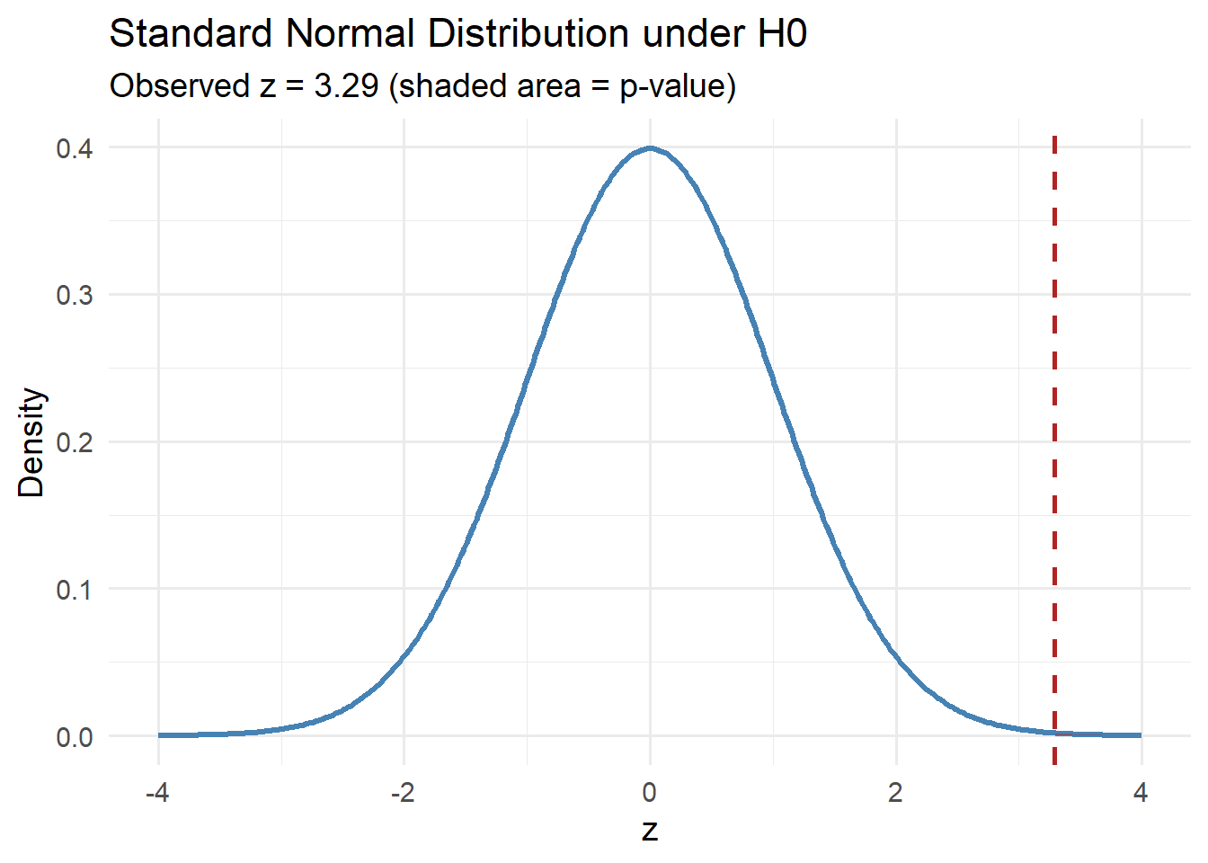
Step 4: \(p\)-value

\[ p = 1 - \Phi(3.29) \approx 0.0005 \]

Step 5: Decision

Since \(p < 0.10\), reject \(H_0\).

Step 6: Interpret

There is strong evidence that more than half of cadets prefer running.

Problem 2

An instructor believes that the average number of push-ups completed by cadets in two minutes is greater than 70. A random sample of \(n = 25\) cadets had a mean of \(\bar{x} = 74.2\) with a sample standard deviation of \(s = 8.5\).

At the 10% significance level, test the instructor’s claim.

Solution

Step 1: Hypotheses

\(H_0: \mu = 70\)
\(H_A: \mu > 70\)

Step 2: Test Statistic

\[ SE = \frac{s}{\sqrt{n}} = \frac{8.5}{\sqrt{25}} = 1.7 \]

\[ t = \frac{\bar{x} - \mu_0}{SE} = \frac{74.2 - 70}{1.7} \approx 2.47 \]

with \(df = n - 1 = 24\).

Step 3: Distribution & Sketch

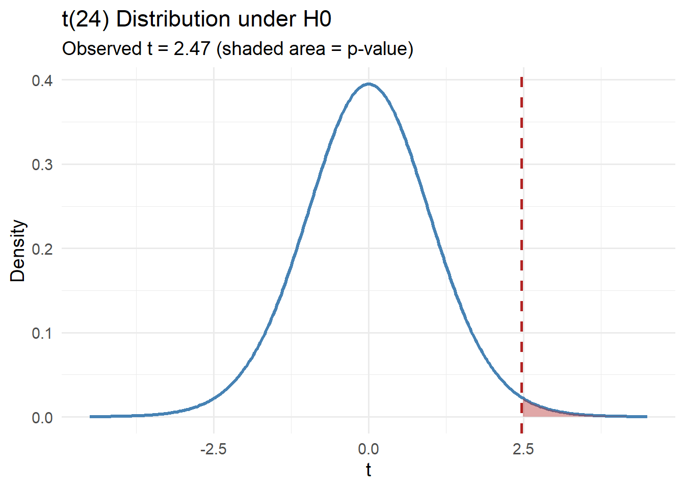
Step 4: \(p\)-value

\[ p = 1 - F_{t_{24}}(2.47) \approx 0.011 \]

Step 5: Decision

Since \(p < 0.10\), reject \(H_0\).

Step 6: Interpret

There is evidence that the true mean number of push-ups is greater than 70.

Intro confidence interval

Before you leave

Today:

Any questions for me?

Upcoming Graded Events

WPR 2: Lesson 22