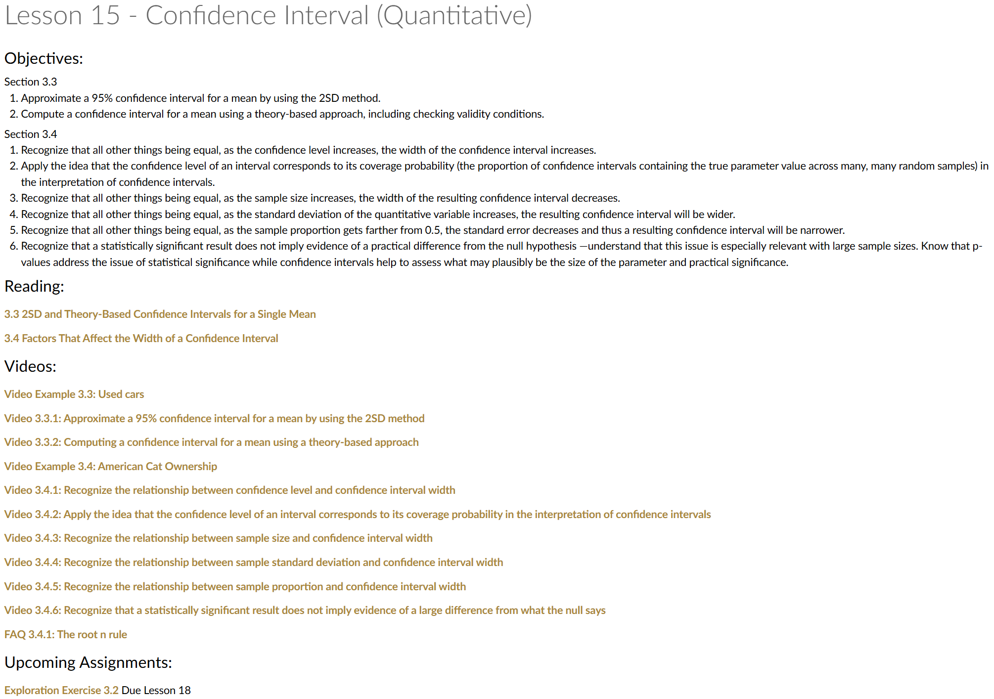
Lesson 15: Confidence Interval (Quantitative)
Lesson Administration
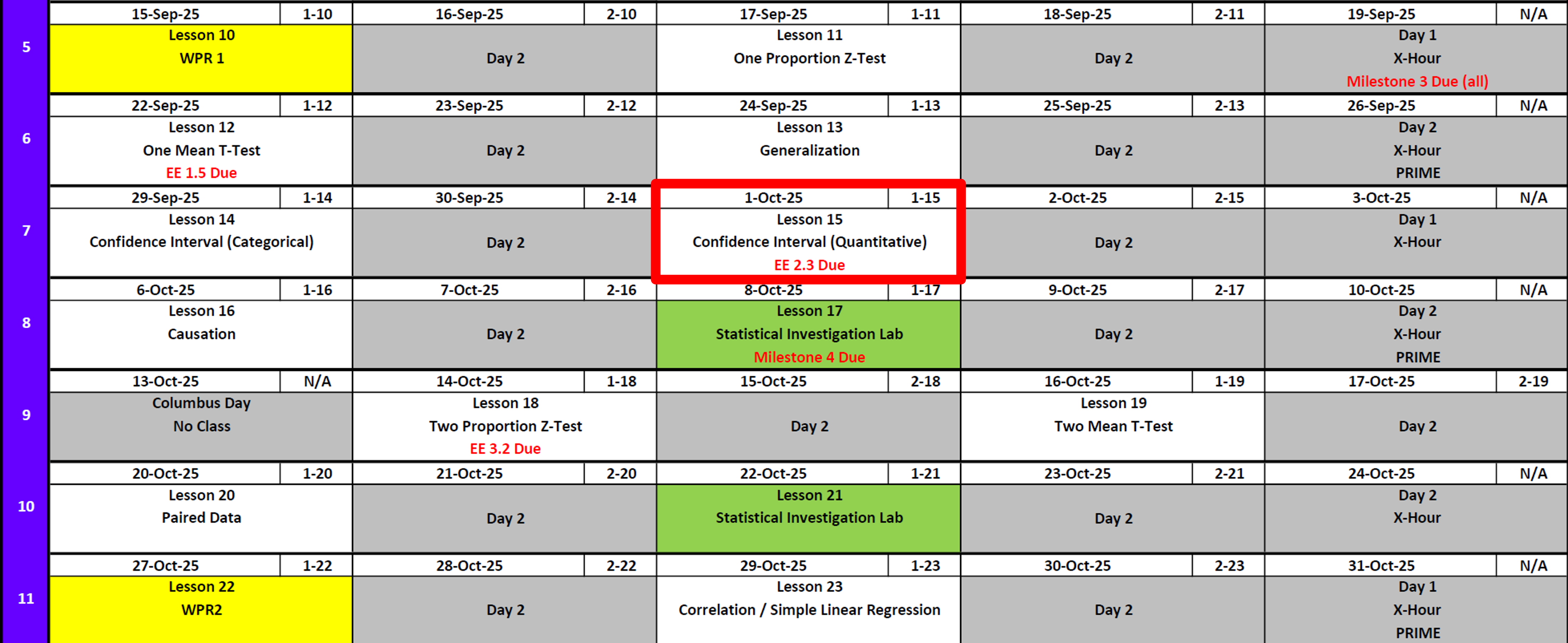
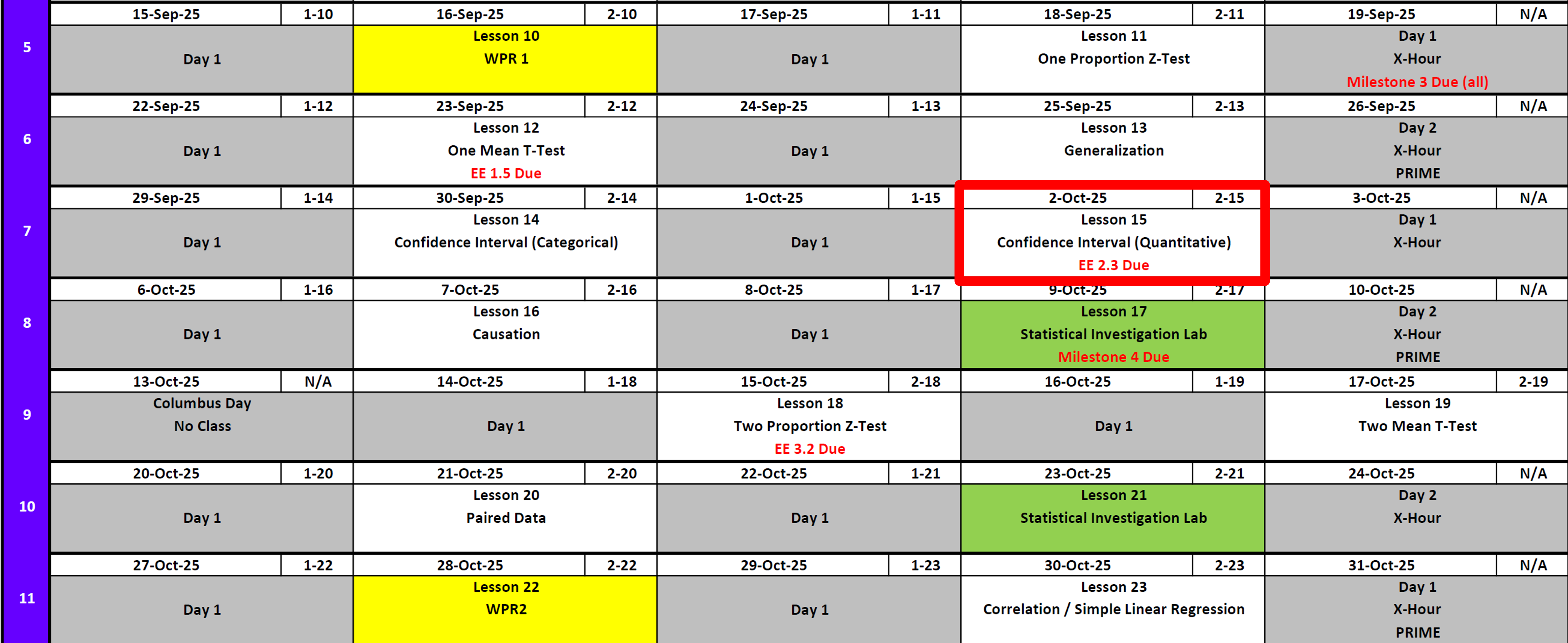
Calendar
Day 1
Day 2
Impact of Government Shut Down
- G1: No Change
- G1: No Change
- I1: Possibly Meet in TH120 but for right now stay put
- J2: No Change
Milestone 4
- Lesson 17
- Milestone 4
- With partner
- Write 1-2 paragraphs per article summarizing the articles topic with a take away for its insight on your project.
- Make updates from Milestone 3 feedback.
- Fill out Annex B for my comments on Milestone 3.
- Turn in EVERYTHING in your working write up.
- Keep your binder up-to-date, but I don’t want to see it.
SIL 1
- Lesson 17
- 25 Points!
- Like a WPR What does that mean?!!
- Read ahead
Exploration Exercise 2.3
- ⏰ Due 0700 on **Lesson 18*
- Lets take a look at it
- Day 1: Tuesday, 14 Oct 2025
- Day 2: Wednesday, 15 Oct 2025
Cal
Things didn’t start well…
But Cal slowly got his act together.

Then he was the first bracket pitcher on the next day against the 2 Seed…

Got the dub:

Lost in the semis vs the eventual champion - not a bad tournament

Reese
We’ll talk about her next lesson!
Review: \(z\)-Tests for One Proportion
For all cases:
\[ z = \frac{\hat{p} - \pi_0}{\sqrt{\frac{\pi_0 (1 - \pi_0)}{n}}} \]
| Alternative Hypothesis | Formula for \(p\)-value | R Code |
|---|---|---|
| \(H_A: p > \pi_0\) | \(p = 1 - \Phi(z)\) | p_val <- 1 - pnorm(z_stat) |
| \(H_A: p < \pi_0\) | \(p = \Phi(z)\) | p_val <- pnorm(z_stat) |
| \(H_A: p \neq \pi_0\) | \(p = 2 \cdot (1 - \Phi(|z|))\) | p_val <- 2 * (1 - pnorm(abs(z_stat))) |
Where:
- \(\hat{p} = R/n\) (sample proportion)
- \(\pi_0\) = hypothesized proportion under \(H_0\)
- \(\Phi(\cdot)\) = cumulative distribution function (CDF) of the standard normal distribution.
Review: \(t\)-Tests for One Mean
For all cases:
\[ t = \frac{\bar{x} - \mu_0}{s / \sqrt{n}} \]
| Alternative Hypothesis | Formula for \(p\)-value | R Code |
|---|---|---|
| \(H_A: \mu > \mu_0\) | \(p = 1 - F_{t_{df}}(t)\) | p_val <- 1 - pt(t_stat, df) |
| \(H_A: \mu < \mu_0\) | \(p = F_{t_{df}}(t)\) | p_val <- pt(t_stat, df) |
| \(H_A: \mu \neq \mu_0\) | \(p = 2 \cdot (1 - F_{t_{df}}(|t|))\) | p_val <- 2 * (1 - pt(abs(t_stat), df)) |
Where:
- \(\bar{x}\) = sample mean
- \(\mu_0\) = hypothesized mean under \(H_0\)
- \(s\) = sample standard deviation
- \(n\) = sample size
- \(df = n - 1\) = degrees of freedom
- \(F_{t_{df}}(\cdot)\) = cumulative distribution function (CDF) of the Student’s \(t\) distribution with \(df\) degrees of freedom
Interpreting the \(p\)-value
Rejecting \(H_0\)
> Since the \(p\)-value is less than \(\alpha\) (e.g., \(0.05\)), we reject the null hypothesis.
> We conclude that there is sufficient evidence to suggest that [state the alternative claim in context].Failing to Reject \(H_0\)
> Since the \(p\)-value is greater than \(\alpha\) (e.g., \(0.05\)), we fail to reject the null hypothesis.
> We conclude that there is not sufficient evidence to suggest that [state the alternative claim in context].
Other Notes
What impacts does altering different values have?
Generalization: We can generalize results to a larger population if the sample is random and representative of that population. Convenience samples don’t justify broad claims.
Causation: We can claim causation only if the study design is a randomized experiment. Observational studies can show associations, but not cause-and-effect.
Parameters vs. Statistics: A parameter is a fixed (but usually unknown) numerical value describing a population (e.g., \(\mu\), \(\sigma\), \(\pi\)). A statistic is a numerical value computed from a sample (e.g., \(\bar{x}\), \(s\), \(\hat{p}\)).
- Parameters = target (what we want to know).
- Statistics = evidence (what we can actually measure).
- We use statistics to estimate parameters, and because different samples give different statistics, we capture this variability with confidence intervals.
- Parameters = target (what we want to know).
| Quantity | Population (Parameter) | Sample (Statistic) |
|---|---|---|
| Center (mean) | \(\mu\) | \(\bar{x}\) |
| Spread (SD) | \(\sigma\) | \(s\) |
| Proportion “success” | \(\pi\) | \(\hat{p}\) |
Confidence Intervals on Means
Suppose we take a random sample of \(n\) cadets and measure a quantitative outcome (e.g., 2-mile run times). We want to estimate the true population mean \(\mu\).
We start with the one-sample \(t\) statistic:
\[ t \;=\; \frac{\bar{x} - \mu_0}{s/\sqrt{n}}. \]
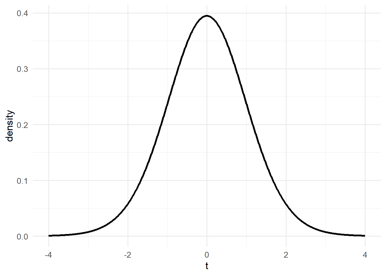
At significance level \(\alpha = 0.05\), we reject \(H_0\) whenever \(t\) falls into the rejection region (the critical tail(s)) of the \(t\) distribution with \(df=n-1\).
Where on this plot would we reject?
Where are these lines?
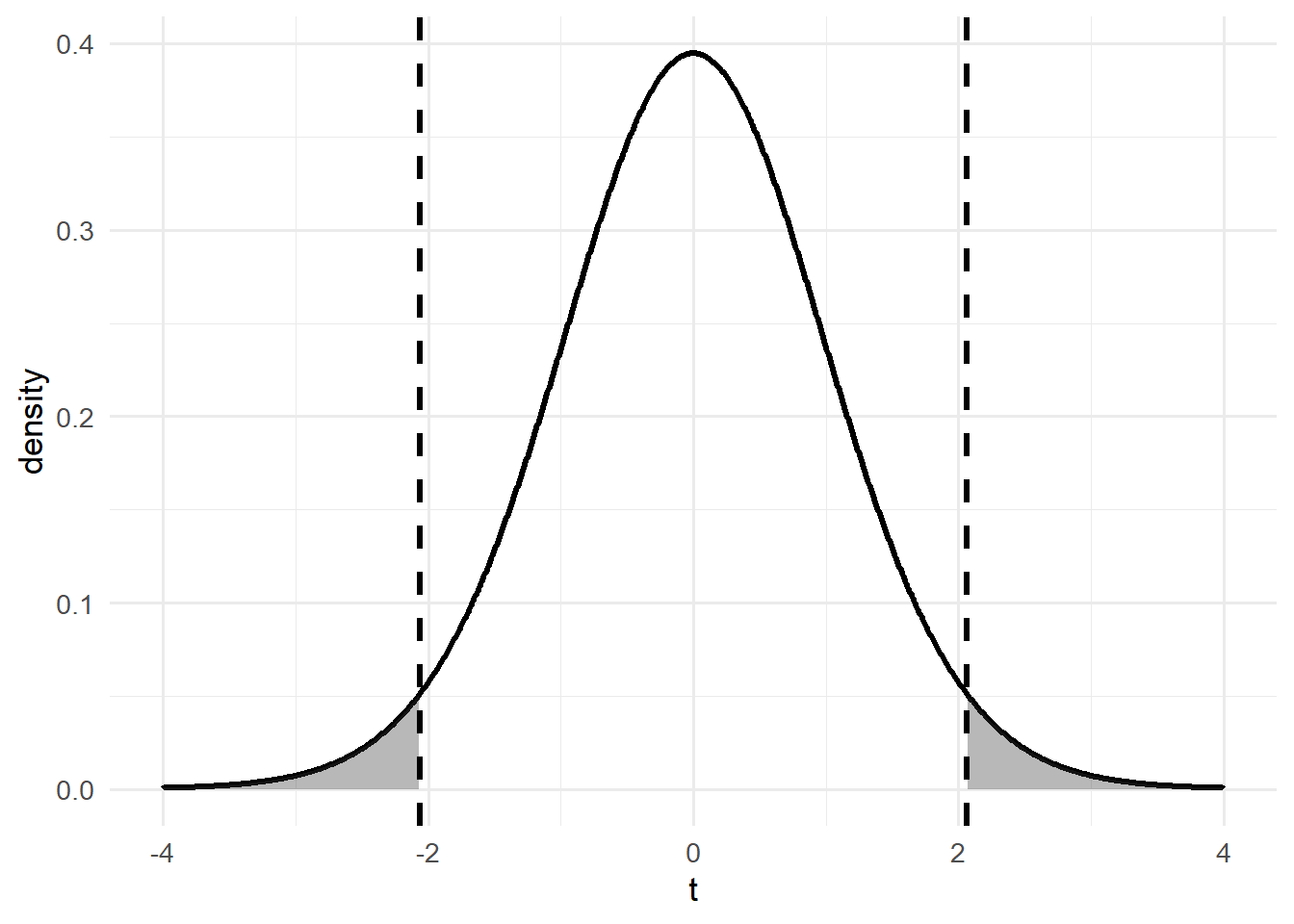
So, the left tail contains \(0.025\) of the distribution, and the right tail contains \(0.025\).
How do we find where \(0.025\) of the distribution is on each side?
We want to solve: \[ 0.025 \;=\; \int_{-\infty}^{x} f_{t,\,df}(z)\,dz, \] where \(f_{t,\,df}\) is the density of the Student’s \(t\) distribution with \(df=n-1\).
When we solve for \(x\), this is the quantile function (inverse CDF).
This integral does not have a simple closed form — that’s why we have R.
qt(0.025, df = df)[1] -2.063899That’s the left cutoff. And the right cutoff:
qt(0.975, df = df)[1] 2.063899So our critical values are about \(-t^\star\) and \(+t^\star\) (here, with \(df=24\), approximately \(\pm 2.064\)).
That is, \[ \pm t^\star \;=\; \frac{\bar{x} - \mu_0}{s/\sqrt{n}}. \]
We don’t know the true \(\mu\), and there isn’t a \(\mu_0\) to plug in for estimation.
So what do we do? We invert the inequality to find the set of \(\mu_0\) values we would not reject:
\[ \bar{x} - \mu_0 \;=\; \pm\, t^\star \cdot \frac{s}{\sqrt{n}} \]
With a little algebra: \[ \begin{align*} \bar{x} - \mu_0 \;&=\; \pm\, t^\star \cdot \frac{s}{\sqrt{n}} \\[6pt] -\mu_0 \;&=\; -\bar{x} \;\pm\; t^\star \cdot \frac{s}{\sqrt{n}} \\[6pt] \mu_0 \;&=\; \bar{x} \;\pm\; t^\star \cdot \frac{s}{\sqrt{n}} \end{align*} \]
So the general 95% confidence interval for a mean is: \[ \bar{x} \;\pm\; t^\star \cdot \frac{s}{\sqrt{n}}, \] with \(t^\star\) taken from the \(t\) distribution with \(df=n-1\).
(Equivalently: the set of \(\mu_0\) values we would not reject at \(\alpha=0.05\).)
Board Problems
Board Problem 1
A random sample of \(n=20\) cadets recorded their 2-mile run times. The sample mean was \(\bar{x} = 13.8\) minutes with a sample standard deviation of \(s = 1.4\) minutes. Assume run times are approximately normal.
- Construct a 90% confidence interval for the true mean run time.
- Construct a 95% confidence interval for the true mean run time.
- Construct a 99% confidence interval for the true mean run time.
NoteSolution
Use the one-sample mean CI: \[ \bar{x}\;\pm\; t^\star \cdot \frac{s}{\sqrt{n}}, \quad df=n-1. \]
Here \(n=20 \Rightarrow df=19\), \(\bar{x}=13.8\), \(s=1.4\).
Compute the \(t^\star\) cutoffs in R (echoed):
df <- 19
qt(0.05, df)  # 90% CI
[1] -1.729133qt(0.025, df) # 95% CI[1] -2.093024qt(0.005, df) # 99% CI[1] -2.86093590% CI: \(13.8 \pm (1.729)\left(\tfrac{1.4}{\sqrt{20}}\right) = 13.8 \pm 0.541 \;\Rightarrow\; [\,13.259,\;14.341\,]\)
95% CI: \(13.8 \pm (2.093)\left(\tfrac{1.4}{\sqrt{20}}\right) = 13.8 \pm 0.655 \;\Rightarrow\; [\,13.145,\;14.455\,]\)
99% CI: \(13.8 \pm (2.861)\left(\tfrac{1.4}{\sqrt{20}}\right) = 13.8 \pm 0.896 \;\Rightarrow\; [\,12.904,\;14.696\,]\)
Board Problem 2
A sample of \(n=15\) cadets reported hours of sleep the night before a training exercise. The sample mean was \(\bar{x} = 6.2\) hours with a sample standard deviation of \(s = 1.1\) hours. Assume sleep hours are approximately normal.
- Construct a 90% confidence interval for the true mean hours of sleep.
- Construct a 95% confidence interval for the true mean hours of sleep.
- Construct a 99% confidence interval for the true mean hours of sleep.
NoteSolution
Use the one-sample mean CI: \[ \bar{x}\;\pm\; t^\star \cdot \frac{s}{\sqrt{n}}, \quad df=n-1. \]
Here \(n=15 \Rightarrow df=14\), \(\bar{x}=6.2\), \(s=1.1\).
Compute the \(t^\star\) cutoffs in R (echoed):
df <- 14
qt(0.05,  df)  # 90% CI
[1] -1.76131qt(0.025, df) # 95% CI[1] -2.144787qt(0.005, df) # 99% CI[1] -2.97684390% CI: \(6.2 \pm (1.761)\left(\tfrac{1.1}{\sqrt{15}}\right) = 6.2 \pm 0.500 \;\Rightarrow\; [\,5.700,\;6.700\,]\)
95% CI: \(6.2 \pm (2.145)\left(\tfrac{1.1}{\sqrt{15}}\right) = 6.2 \pm 0.609 \;\Rightarrow\; [\,5.591,\;6.809\,]\)
99% CI: \(6.2 \pm (2.977)\left(\tfrac{1.1}{\sqrt{15}}\right) = 6.2 \pm 0.846 \;\Rightarrow\; [\,5.354,\;7.046\,]\)
Board Problem 3
In a random sample of \(n=240\) respondents, \(x=102\) reported using public transit at least once per week.
- Construct a 90% confidence interval for the true proportion who use public transit weekly.
- Construct a 95% confidence interval for the true proportion.
- Construct a 99% confidence interval for the true proportion.
NoteSolution
Use the confidence interval for a proportion: \[ \hat{p}\;\pm\; z^\star \sqrt{\frac{\hat{p}\,(1-\hat{p})}{n}},\qquad \hat{p}=\frac{x}{n}. \]
Here, \(\hat{p}=\dfrac{102}{240}=0.425\) and \(n=240\).
Compute the \(z^\star\) cutoffs in R:
n <- 240; x <- 102
phat <- x/n
z90 <- qnorm(0.95)   # for 90% CI
z95 <- qnorm(0.975)  # for 95% CI
z99 <- qnorm(0.995)  # for 99% CI
z90; z95; z99
[1] 1.644854[1] 1.959964[1] 2.57582990% CI: \[ 0.425 \;\pm\; (1.645)\sqrt{\frac{0.425(1-0.425)}{240}} \;=\; 0.425 \pm 0.052 \;\Rightarrow\; [\,0.373,\;0.477\,]. \]
95% CI: \[ 0.425 \;\pm\; (1.960)\sqrt{\frac{0.425(1-0.425)}{240}} \;=\; 0.425 \pm 0.063 \;\Rightarrow\; [\,0.362,\;0.488\,]. \]
99% CI: \[ 0.425 \;\pm\; (2.576)\sqrt{\frac{0.425(1-0.425)}{240}} \;=\; 0.425 \pm 0.082 \;\Rightarrow\; [\,0.343,\;0.507\,]. \]
Board Problem 4
A random sample of \(n=30\) cadets was asked how many push-ups they could complete in two minutes. The sample mean was \(\bar{x} = 58.5\) with a sample standard deviation of \(s = 9.3\). Assume counts are approximately normal.
- Construct a 90% confidence interval for the true mean number of push-ups.
- Construct a 95% confidence interval for the true mean number of push-ups.
- Construct a 99% confidence interval for the true mean number of push-ups.
NoteSolution
Use the one-sample mean CI: \[ \bar{x}\;\pm\; t^\star \cdot \frac{s}{\sqrt{n}}, \quad df=n-1. \]
Here \(n=30 \Rightarrow df=29\), \(\bar{x}=58.5\), \(s=9.3\).
Compute the \(t^\star\) cutoffs in R (echoed):
df <- 29
qt(0.05, df)  # 90% CI
[1] -1.699127qt(0.025, df) # 95% CI[1] -2.04523qt(0.005, df) # 99% CI[1] -2.75638690% CI: \(58.5 \pm (1.699)\left(\tfrac{9.3}{\sqrt{30}}\right) = 58.5 \pm 2.884 \;\Rightarrow\; [\,55.616,\;61.384\,]\)
95% CI: \(58.5 \pm (2.045)\left(\tfrac{9.3}{\sqrt{30}}\right) = 58.5 \pm 3.471 \;\Rightarrow\; [\,55.029,\;61.971\,]\)
99% CI: \(58.5 \pm (2.756)\left(\tfrac{9.3}{\sqrt{30}}\right) = 58.5 \pm 4.676 \;\Rightarrow\; [\,53.824,\;63.176\,]\)
Before you leave
Today:
- Any questions for me?
Upcoming Graded Events
- WPR 2: Lesson 22