Lesson 23: Correlation & Simple Linear Regression

Lesson Administration

Calendar

Day 1

Day 2

SIL 2 Points

Milestone 5

Lesson 25.5
7 November
Milestone 5 Instructions

Exploration Exercise 4.4

Lesson 26
12-13 November
Link: TBD

Milestone 6: Draft Tech Report

Lesson 26.5
17 November
Milestone 6 Instructions

Project Presentations

Milestone 7

Milestone 8

TEE Times

Date	Start	End
Wed, 17 Dec 2025	1300	1630
Thu, 18 Dec 2025	0730	1100

Cal

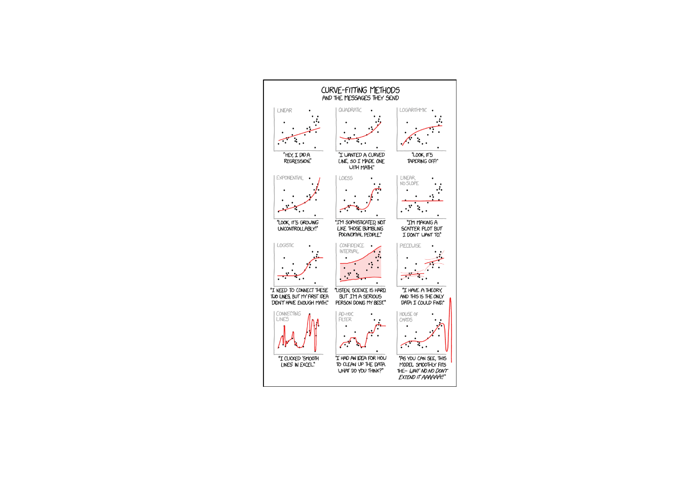
Linear Regression

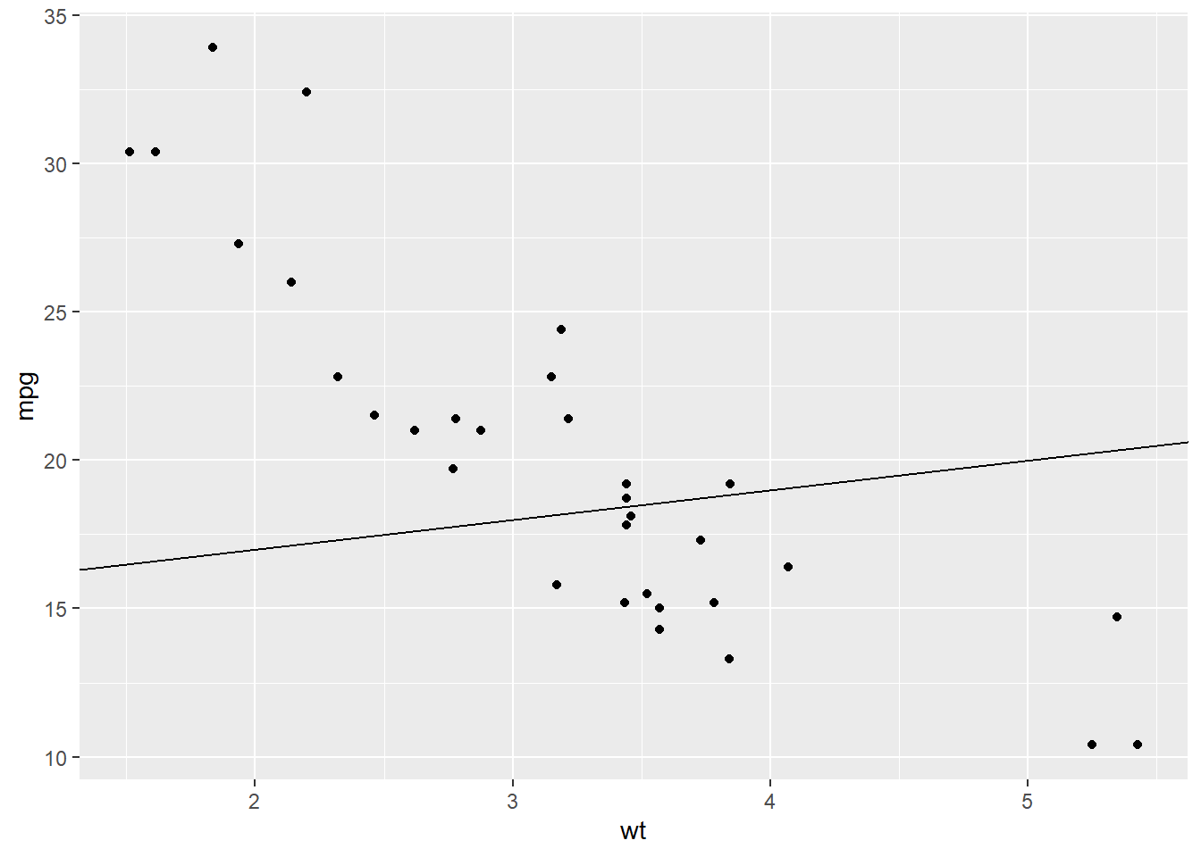
We can see a clear trend here from weight to miles per gallon:

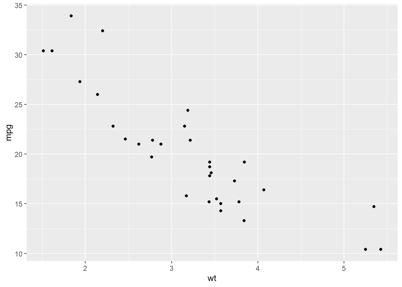
There should be some type of y = mx + b formula that could help us model this relationship or predict a new point in here somewhere.

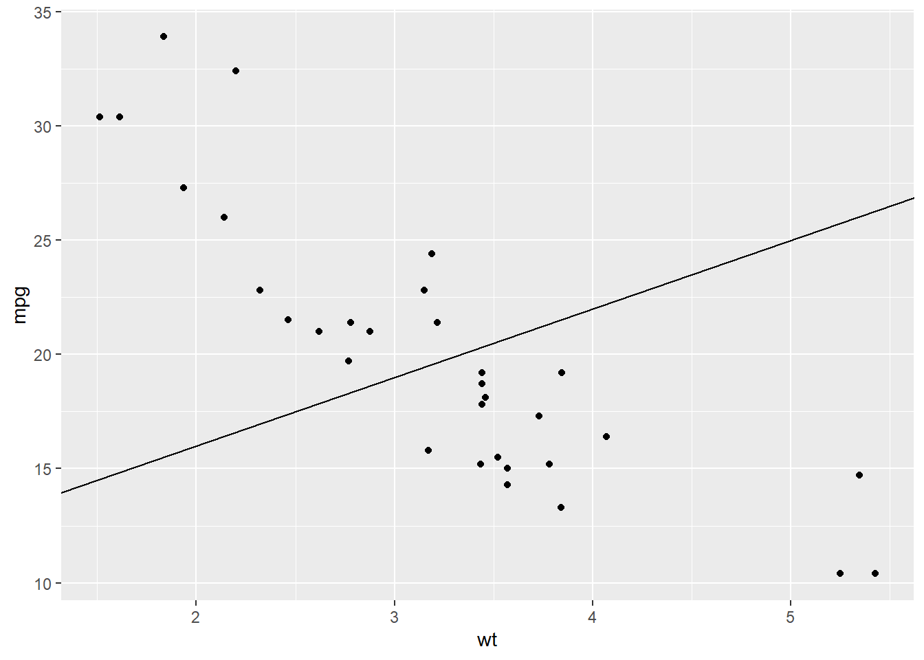
What about this one?

Or this one?

Or this one?

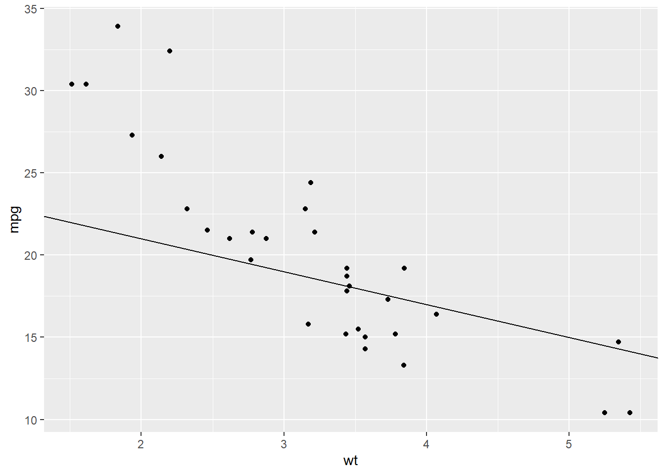
Are these lines good? Are these lines good enough? Are these lines the best?

Wouldn’t it be nice if we could mathematically decide what the best line is for this?

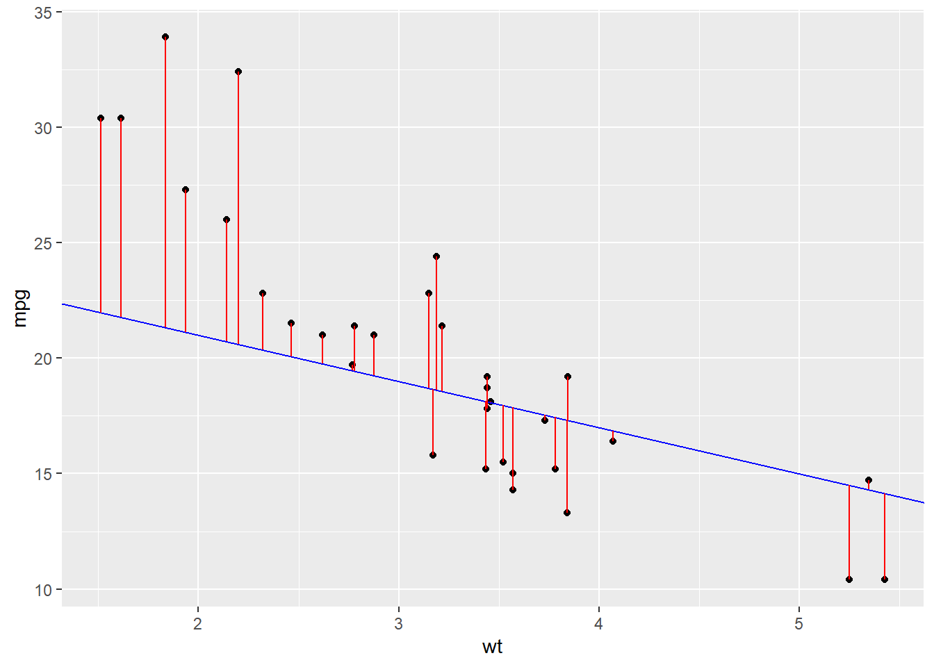
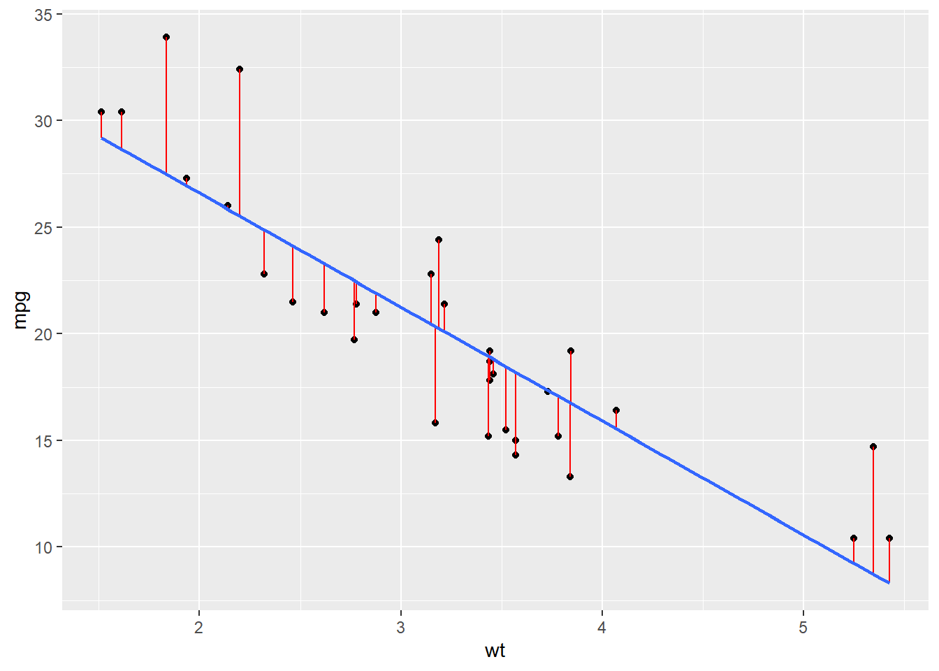
How would we do that? The idea is that a best line would minimize the red lines in this plot.

How Do We Find the Best Line?

We just saw that some lines fit the data better than others. But we need a mathematical way to decide what “best” means.

Step 1: Define the Residual (Error)

For each point \((x_i, y_i)\), the line makes a prediction:

\[ \hat{y}_i = \beta_0 + \beta_1 x_i \]

The error (residual) is the difference between the actual \(y_i\) and the predicted \(\hat{y}_i\):

\[ \begin{align*} e_i &= y_i - \hat{y}_i \\ &= y_i - (\beta_0 + \beta_1 x_i) \\ &= y_i - \beta_0 - \beta_1 x_i \end{align*} \]

Step 2: Define the Loss Function (Sum of Squared Errors)

We want all the errors to be as small as possible. But errors can be positive or negative, so we square them and add them up:

\[ S(\beta_0, \beta_1) = \sum_{i=1}^n e_i^2 = \sum_{i=1}^n \left(y_i - \beta_0 - \beta_1 x_i\right)^2 \]

This function \(S(\beta_0, \beta_1)\) is our loss function. The “best” line is the one that makes this sum as small as possible.

Step 3: Minimize with Calculus

We take partial derivatives of \(S\) with respect to \(\beta_0\) and \(\beta_1\), set them to zero, and solve.

Derivative with respect to \(\beta_0\):

\[ \begin{align*} \frac{\partial S}{\partial \beta_0} &= -2\sum_{i=1}^n \left(y_i - \beta_0 - \beta_1 x_i\right) = 0 \\[6pt] &= \sum_{i=1}^n \left(y_i - \beta_0 - \beta_1 x_i\right) = 0 \\[6pt] &= \sum_{i=1}^n y_i - \sum_{i=1}^n \beta_0 - \sum_{i=1}^n \beta_1x_i \\[6pt] &= \sum_{i=1}^n y_i - n\beta_0 - \beta_1 \sum_{i=1}^n x_i \\[6pt] n\beta_0 &= \sum_{i=1}^n y_i - \beta_1 \sum_{i=1}^n x_i \\[6pt] \beta_0 &= \frac{1}{n}\sum_{i=1}^n y_i - \beta_1 \frac{1}{n}\sum_{i=1}^n x_i \\[6pt] \beta_0 &= \bar{y} - \beta_1 \bar{x}. \end{align*} \]

Derivative with respect to \(\beta_1\):

\[ \begin{align*} \frac{\partial S}{\partial \beta_1} &= -2\sum_{i=1}^n x_i\left(y_i - \beta_0 - \beta_1 x_i\right) = 0 \\[6pt] &= \sum_{i=1}^n \left(x_i y_i - \beta_0 x_i - \beta_1 x_i^2\right) = 0 \\[6pt] &= \sum_{i=1}^n x_i y_i \;-\; \beta_0 \sum_{i=1}^n x_i \;-\; \beta_1 \sum_{i=1}^n x_i^2 = 0 \\[6pt] &= \sum_{i=1}^n x_i y_i \;-\; (\bar y - \beta_1 \bar x)\sum_{i=1}^n x_i \;-\; \beta_1 \sum_{i=1}^n x_i^2 = 0 \\[6pt] &= \sum_{i=1}^n x_i y_i \;-\; (\bar y - \beta_1 \bar x)n \bar x \;-\; \beta_1 \sum_{i=1}^n x_i^2 = 0 \\[6pt] &= \sum_{i=1}^n x_i y_i \;-\; n\bar x \bar y \;+\; \beta_1 n \bar x^2 \;-\; \beta_1 \sum_{i=1}^n x_i^2 = 0 \\[6pt] \beta_1\!\left(\sum_{i=1}^n x_i^2 - n\bar x^2\right) &= \sum_{i=1}^n x_i y_i - n\bar x \bar y \\[6pt] \beta_1 &= \dfrac{\sum_{i=1}^n x_i y_i - n\bar x \bar y}{\sum_{i=1}^n x_i^2 - n\bar x^2} \\[6pt] \beta_1 &= \dfrac{\sum_{i=1}^n x_i y_i - n\bar x \bar y - n\bar x \bar y + n\bar x \bar y}{\sum_{i=1}^n x_i^2 - n\bar x^2 - 2 n \bar x \bar x + 2 n \bar x \bar x} \\[6pt] \beta_1 &= \dfrac{\sum_{i=1}^n x_i y_i - \bar x (n \bar y) - \bar y (n\bar x) + n\bar x \bar y}{\sum_{i=1}^n x_i^2 - n\bar x^2 - 2 \bar x (n \bar x) + 2 n \bar x^2} \\[6pt] \beta_1 &= \dfrac{\sum_{i=1}^n x_i y_i - \bar x \sum_{i=1}^n y_i - \bar y \sum_{i=1}^n x_i + n\bar x \bar y}{\sum_{i=1}^n x_i^2 - n\bar x^2 - 2\bar x \sum_{i=1}^n x_i + 2n\bar x^2} \\[6pt] \beta_1 &= \dfrac{\sum_{i=1}^n (x_i y_i - \bar x y_i - \bar y x_i + \bar x \bar y)}{\sum_{i=1}^n x_i^2 - 2\bar x \sum_{i=1}^n x_i + n\bar x^2} \\[6pt] \beta_1 &= \dfrac{\sum_{i=1}^n (x_i-\bar x)(y_i-\bar y)}{\sum_{i=1}^n x_i^2 - 2\bar x \sum_{i=1}^n x_i + \sum_{i=1}^n \bar x^2} \\[6pt] \beta_1 &= \dfrac{\sum_{i=1}^n (x_i-\bar x)(y_i-\bar y)}{\sum_{i=1}^n x_i^2 - 2\bar x x_i + \bar x^2} \\[6pt] \beta_1 &= \dfrac{\sum_{i=1}^n (x_i-\bar x)(y_i-\bar y)}{\sum_{i=1}^n (x_i-\bar x)^2}. \end{align*} \]

So to sum it up:

\[ \begin{aligned} \beta_1 &= \dfrac{\sum_{i=1}^n (x_i - \bar x)(y_i - \bar y)}{\sum_{i=1}^n (x_i - \bar x)^2} \\[6pt] \beta_0 &= \bar y - \beta_1 \bar x \end{aligned} \]

Step 4: Interpretation

\[ \hat{y}_i = \beta_0 + \beta_1 x_i \]

\(\hat{\beta}_1\) is the slope — how much \(y\) changes on average when \(x\) increases by 1.
\(\hat{\beta}_0\) is the intercept — the value of \(y\) when \(x = 0\).

So remember this plot?

These formulas guarantee that our line is the one that minimizes the red “error bars”.

Regression Equation

lm(formula = mpg~wt, data = mtcars)


Call:
lm(formula = mpg ~ wt, data = mtcars)

Coefficients:
(Intercept)           wt  
     37.285       -5.344

So this means

\[ \widehat{mpg} \;=\; 37.39 \;-\; 5.34 \, wt \]

Interpretation

Intercept (37.39): If a car had zero weight (not realistic, but useful mathematically), the predicted mpg would be 37.39.
Slope (-5.34): For each additional 1000 lbs of weight, the predicted fuel efficiency decreases on average by about 5.3 mpg.

Significance

How do we know if we can “trust” our slope coefficient, \(\beta_1\)?

We frame this as a hypothesis test:

\[ H_0: \; \beta_1 = 0 \quad \text{(no linear relationship)} \]

\[ H_A: \; \beta_1 \neq 0 \quad \text{(some linear relationship exists)} \]

mod <- lm(mpg ~ wt, data = mtcars)
summary(mod)


Call:
lm(formula = mpg ~ wt, data = mtcars)

Residuals:
    Min      1Q  Median      3Q     Max 
-4.5432 -2.3647 -0.1252  1.4096  6.8727 

Coefficients:
            Estimate Std. Error t value Pr(>|t|)    
(Intercept)  37.2851     1.8776  19.858  < 2e-16 ***
wt           -5.3445     0.5591  -9.559 1.29e-10 ***
---
Signif. codes:  0 '***' 0.001 '**' 0.01 '*' 0.05 '.' 0.1 ' ' 1

Residual standard error: 3.046 on 30 degrees of freedom
Multiple R-squared:  0.7528,    Adjusted R-squared:  0.7446 
F-statistic: 91.38 on 1 and 30 DF,  p-value: 1.294e-10

For a little more depth

The test statistic here is calculated as

\[ t = \frac{\beta_1 - \text{null}}{SE} = \frac{37.2851}{1.8776} = 19.858 \]

And if you remember…

2 * (1 - pt(abs(19.858), 32))

[1] 0

Model Fit

How good is this model? One way to measure it is with the coefficient of determination:

\[ R^2 = 0.7528 \]

This means that about 75% of the variation in mpg can be explained by the linear relationship with car weight.
The remaining 25% of the variation is due to other factors not captured by this model (such as horsepower, number of cylinders, transmission type, etc.).

Key Point

A high \(R^2\) (close to 1) means the model explains a lot of the variation.
A low \(R^2\) (close to 0) means the model doesn’t explain much variation.
Here, \(R^2 = 0.75\) suggests the model is quite strong for such a simple one-variable regression.

Board Problem

Do this regression for mpg against hp, drat, and disp.

Report the regression equation.
State the hypothesis test and conclusion.
Decide if each variable has a linear relationship with mpg.
Finally, which model is best when it comes to explaining mpg? Why?

                   mpg cyl disp  hp drat    wt  qsec vs am gear carb
Mazda RX4         21.0   6  160 110 3.90 2.620 16.46  0  1    4    4
Mazda RX4 Wag     21.0   6  160 110 3.90 2.875 17.02  0  1    4    4
Datsun 710        22.8   4  108  93 3.85 2.320 18.61  1  1    4    1
Hornet 4 Drive    21.4   6  258 110 3.08 3.215 19.44  1  0    3    1
Hornet Sportabout 18.7   8  360 175 3.15 3.440 17.02  0  0    3    2
Valiant           18.1   6  225 105 2.76 3.460 20.22  1  0    3    1

Solution

Step 1: Fit the regression models


Call:
lm(formula = mpg ~ hp, data = mtcars)

Residuals:
    Min      1Q  Median      3Q     Max 
-5.7121 -2.1122 -0.8854  1.5819  8.2360 

Coefficients:
            Estimate Std. Error t value Pr(>|t|)    
(Intercept) 30.09886    1.63392  18.421  < 2e-16 ***
hp          -0.06823    0.01012  -6.742 1.79e-07 ***
---
Signif. codes:  0 '***' 0.001 '**' 0.01 '*' 0.05 '.' 0.1 ' ' 1

Residual standard error: 3.863 on 30 degrees of freedom
Multiple R-squared:  0.6024,    Adjusted R-squared:  0.5892 
F-statistic: 45.46 on 1 and 30 DF,  p-value: 1.788e-07

Model 1 (hp):
\[\widehat{mpg}=30.10-0.07\,hp\]

\(H_0:\;\beta_1=0 \quad \text{(no linear relationship)}\)
\(H_A:\;\beta_1\neq 0 \quad \text{(linear relationship exists)}\)

\(p<0.001\) → reject \(H_0\), horsepower is significantly related to mpg.
\(R^2=0.602\) → explains ~60% of variation.


Call:
lm(formula = mpg ~ drat, data = mtcars)

Residuals:
    Min      1Q  Median      3Q     Max 
-9.0775 -2.6803 -0.2095  2.2976  9.0225 

Coefficients:
            Estimate Std. Error t value Pr(>|t|)    
(Intercept)   -7.525      5.477  -1.374     0.18    
drat           7.678      1.507   5.096 1.78e-05 ***
---
Signif. codes:  0 '***' 0.001 '**' 0.01 '*' 0.05 '.' 0.1 ' ' 1

Residual standard error: 4.485 on 30 degrees of freedom
Multiple R-squared:  0.464, Adjusted R-squared:  0.4461 
F-statistic: 25.97 on 1 and 30 DF,  p-value: 1.776e-05

Model 2 (drat):
\[\widehat{mpg}=-7.52+7.68\,drat\]

\(H_0:\;\beta_1=0 \quad \text{(no linear relationship)}\)
\(H_A:\;\beta_1\neq 0 \quad \text{(linear relationship exists)}\)

\(p<0.001\) → reject \(H_0\), drat is significantly related to mpg.
\(R^2=0.464\) → explains ~46% of variation.


Call:
lm(formula = mpg ~ disp, data = mtcars)

Residuals:
    Min      1Q  Median      3Q     Max 
-4.8922 -2.2022 -0.9631  1.6272  7.2305 

Coefficients:
             Estimate Std. Error t value Pr(>|t|)    
(Intercept) 29.599855   1.229720  24.070  < 2e-16 ***
disp        -0.041215   0.004712  -8.747 9.38e-10 ***
---
Signif. codes:  0 '***' 0.001 '**' 0.01 '*' 0.05 '.' 0.1 ' ' 1

Residual standard error: 3.251 on 30 degrees of freedom
Multiple R-squared:  0.7183,    Adjusted R-squared:  0.709 
F-statistic: 76.51 on 1 and 30 DF,  p-value: 9.38e-10

Model 3 (disp):
\[\widehat{mpg}=29.60-0.04\,disp\]

\(H_0:\;\beta_1=0 \quad \text{(no linear relationship)}\)
\(H_A:\;\beta_1\neq 0 \quad \text{(linear relationship exists)}\)

\(p<0.001\) → reject \(H_0\), displacement is significantly related to mpg.
\(R^2=0.718\) → explains ~72% of variation.

Step 2: Compare models

All three predictors (hp, drat, disp) show significant evidence of a linear relationship with mpg.
Among them, displacement (disp) has the highest \(R^2\) (0.718), meaning it explains the most variation in mpg.
Therefore, the simple regression with displacement is the best single-variable model for predicting mpg in this dataset.

Answer: Displacement (\(disp\)) gives the best simple linear regression model for mpg because it explains the largest proportion of variation (\(R^2=0.72\)).

Lesson 23: Correlation & Simple Linear Regression

Lesson Administration

Calendar

Day 1

Day 2

SIL 2 Points

Milestone 5

Exploration Exercise 4.4

Milestone 6: Draft Tech Report

Project Presentations

Milestone 7

Milestone 8

TEE Times

Cal

Linear Regression

How Do We Find the Best Line?

Step 1: Define the Residual (Error)

Step 2: Define the Loss Function (Sum of Squared Errors)

Step 3: Minimize with Calculus

Step 4: Interpretation

Regression Equation

Significance

Model Fit

Board Problem

Before you leave

Today:

Upcoming Graded Events