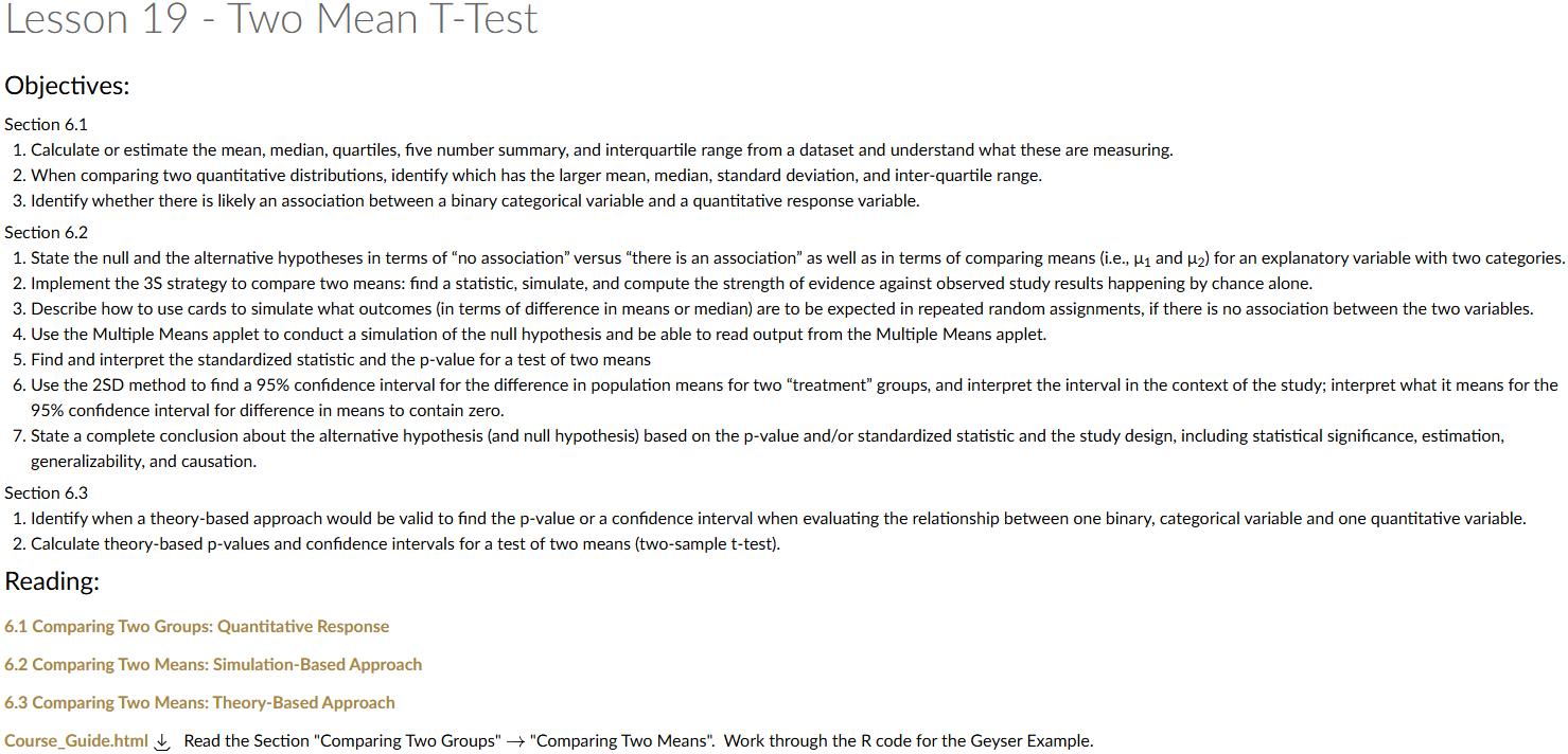
Lesson 19: Two Mean T-Test

Lesson Administration

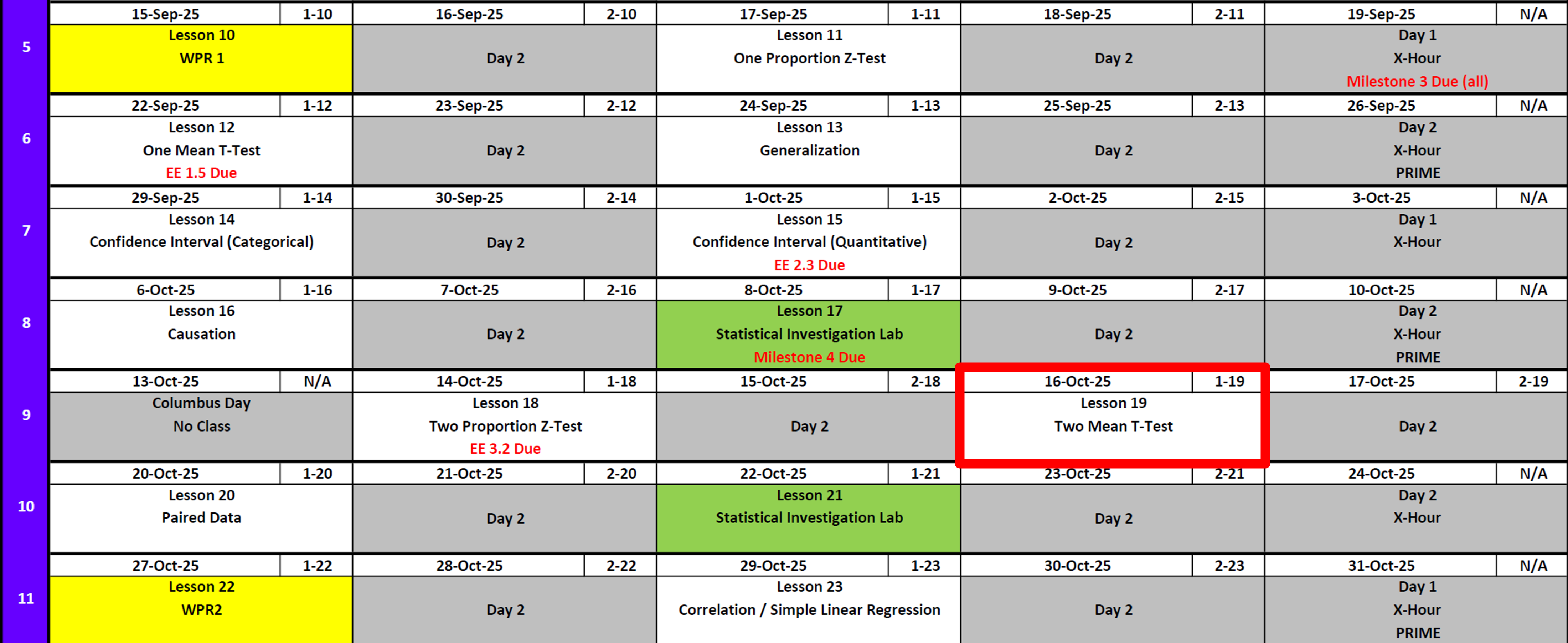
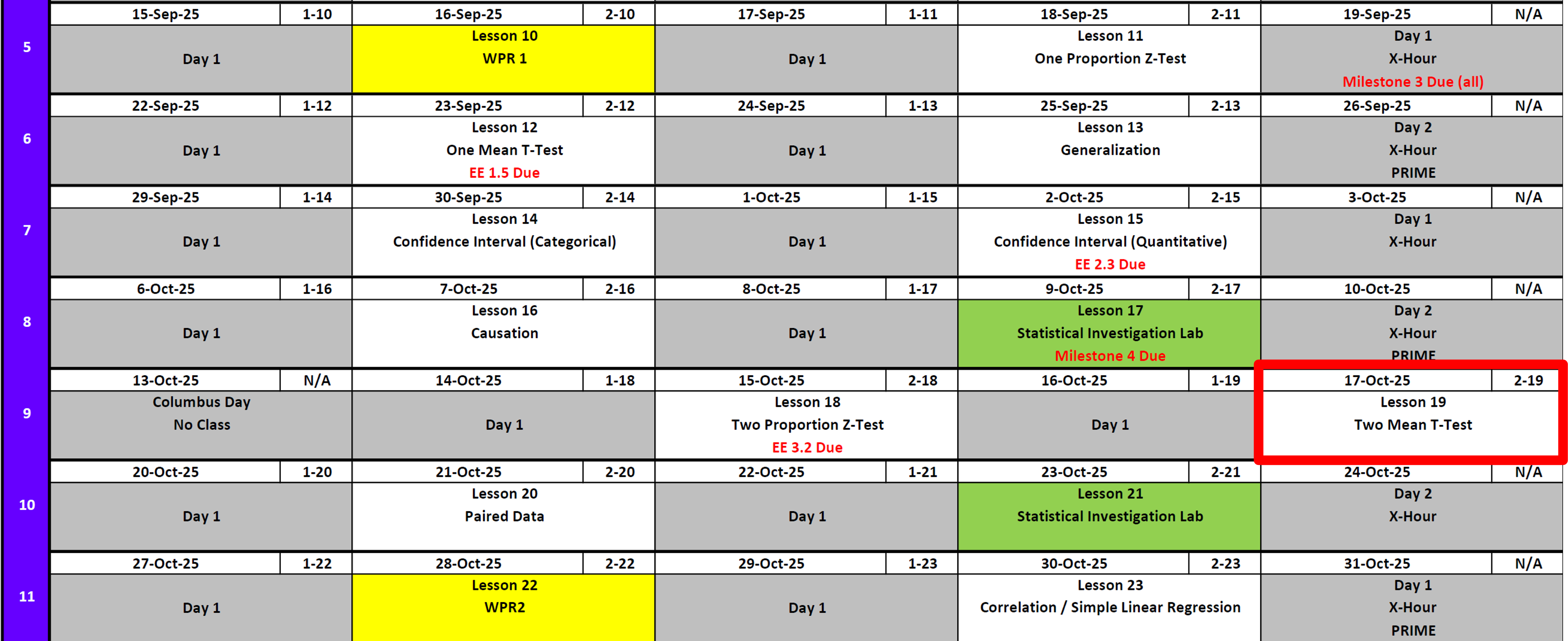
Calendar

Day 1

Day 2

SIL 1 (Redeployment)

• What it means for you depending on how you feel about it

Exploration Exercise 3.2 (Next Lesson - HARD COPY!!)

• ⏰ Due on Lesson 19 (Today)
  
  • Day 1: Tuesday, 16 Oct 2025
  • Day 2: Wednesday, 17 Oct 2025

Exploration Exercise 7.2

• Canvas Quiz Due 21 OCT at Midnight

SIL 2

• Details
• Shorter version of last time with in class feedback time

WPR 2

Milestone 5

• Due 0700 on 7 November
• Instructions

DMath Frisbee PLAYOFFS!!

Math 1 vs DPE

NotePreviously 5-0

6-0

Army Math

Cal

Running Review

Review: \(z\)-Tests for One Proportion

For all cases:

\(H_0:\ \pi = \pi_0\)

\[ z = \frac{\hat{p} - \pi_0}{\sqrt{\frac{\hat{p}\,(1-\hat{p})}{n}}} \]

Alternative Hypothesis	Formula for \(p\)-value	R Code
\(H_A:\ \pi > \pi_0\)	\(p = 1 - \Phi(z)\)	p_val <- 1 - pnorm(z_stat)
\(H_A:\ \pi < \pi_0\)	\(p = \Phi(z)\)	p_val <- pnorm(z_stat)
\(H_A:\ \pi \neq \pi_0\)	\(p = 2 \cdot (1 - \Phi(|z|))\)	p_val <- 2 * (1 - pnorm(abs(z_stat)))

Where:

• \(\hat{p} = R/n\) (sample proportion)
  
• \(\pi_0\) = hypothesized proportion under \(H_0\)
  
• \(\Phi(\cdot)\) = cumulative distribution function (CDF) of the standard normal distribution

Validity Conditions

• Number of successes and failures must be greater than 10.

Confidence Interval for \(\pi\) (one proportion)

\[ \hat{p} \;\pm\; z_{\,1-\alpha/2}\,\sqrt{\frac{\hat{p}\,(1-\hat{p})}{n}} \]

I am \((1 - \alpha)\%\) confident that the true population proportion \(\pi\) lies between \([\text{lower bound}, \text{upper bound}]\).

---

Review: \(t\)-Tests for One Mean

For all cases:

\(H_0:\ \mu = \mu_0\)

\[ t = \frac{\bar{x} - \mu_0}{s / \sqrt{n}} \]

Alternative Hypothesis	Formula for \(p\)-value	R Code
\(H_A:\ \mu > \mu_0\)	\(p = 1 - F_{t,df}(t)\)	p_val <- 1 - pt(t_stat, df)
\(H_A:\ \mu < \mu_0\)	\(p = F_{t,df}(t)\)	p_val <- pt(t_stat, df)
\(H_A:\ \mu \neq \mu_0\)	\(p = 2 \cdot (1 - F_{t,df}(|t|))\)	p_val <- 2 * (1 - pt(abs(t_stat), df))

Where:

• \(\bar{x}\) = sample mean
  
• \(\mu_0\) = hypothesized mean under \(H_0\)
  
• \(s\) = sample standard deviation
  
• \(n\) = sample size
  
• \(df = n - 1\) (degrees of freedom)
  
• \(F_{t,df}(\cdot)\) = CDF of Student’s \(t\) distribution with \(df\) degrees of freedom

Validity Conditions

• Sample size must be greater than 30.

Confidence Interval for \(\mu\) (one mean)

\[ \bar{x} \;\pm\; t_{\,1-\alpha/2,\;df}\,\frac{s}{\sqrt{n}}, \qquad df = n-1 \] I am \((1 - \alpha)\%\) confident that the true population mean \((\mu)\) lies between \([\text{lower bound}, \text{upper bound}]\).

---

Review: \(z\)-Tests for Two Proportions

For all cases:

\(H_0:\ \pi_1 - \pi_2 = 0\)

\[ z \;=\; \frac{(\hat{p}_1 - \hat{p}_2) - (\pi_1 - \pi_2)}{\sqrt{\hat{p}(1-\hat{p})\left(\tfrac{1}{n_1} + \tfrac{1}{n_2}\right)}} \]

Where the pooled proportion is

\[ \hat{p} \;=\; \frac{x_1 + x_2}{n_1 + n_2}. \]

Alternative Hypothesis	Formula for \(p\)-value	R Code
\(H_A:\ \pi_1 - \pi_2 > 0\)	\(p = 1 - \Phi(z)\)	p_val <- 1 - pnorm(z_stat)
\(H_A:\ \pi_1 - \pi_2 < 0\)	\(p = \Phi(z)\)	p_val <- pnorm(z_stat)
\(H_A:\ \pi_1 - \pi_2 \neq 0\)	\(p = 2 \cdot (1 - \Phi(|z|))\)	p_val <- 2 * (1 - pnorm(abs(z_stat)))

Where:

• \(\hat{p}_1 = x_1/n_1\) (sample proportion in group 1)
  
• \(\hat{p}_2 = x_2/n_2\) (sample proportion in group 2)
  
• \(\pi_1, \pi_2\) = hypothesized proportions under \(H_0\)
  
• \(\Phi(\cdot)\) = cumulative distribution function (CDF) of the standard normal distribution

Validity Conditions

• Each group must have at least 10 successes and 10 failures.

Confidence Interval for \(\pi_1 - \pi_2\) (unpooled SE)

\[ (\hat{p}_1 - \hat{p}_2) \;\pm\; z_{\,1-\alpha/2}\, \sqrt{\tfrac{\hat{p}_1(1-\hat{p}_1)}{n_1} + \tfrac{\hat{p}_2(1-\hat{p}_2)}{n_2}} \]

I am \((1 - \alpha)\%\) confident that the true difference in population proportions \((\pi_1 - \pi_2)\) lies between \([\text{lower bound}, \text{upper bound}]\).

---

Interpreting the \(p\)-value

• Rejecting \(H_0\)
  > Since the \(p\)-value is less than \(\alpha\) (e.g., \(0.05\)), we reject the null hypothesis.
  > We conclude that there is sufficient evidence to suggest that [state the alternative claim in context].

• Failing to Reject \(H_0\)
  > Since the \(p\)-value is greater than \(\alpha\) (e.g., \(0.05\)), we fail to reject the null hypothesis.
  > We conclude that there is not sufficient evidence to suggest that [state the alternative claim in context].

• Strength of evidence: Smaller \(p\) means stronger evidence against \(H_0\).

Other Notes

• Generalization: We can generalize results to a larger population if the data come from a random and representative sample of that population.
  
• Causation: We can claim causation if participants are randomly assigned to treatments in an experiment. Without random assignment, we can only conclude association, not causation.

\[ \begin{array}{|c|c|c|} \hline & \text{Randomly Sampled} & \text{Not Randomly Sampled} \\ \hline \textbf{Randomly Assigned} & \begin{array}{c} \text{Generalize: Yes} \\ \text{Causation: Yes} \end{array} & \begin{array}{c} \text{Generalize: No} \\ \text{Causation: Yes} \end{array} \\ \hline \textbf{Not Randomly Assigned} & \begin{array}{c} \text{Generalize: Yes} \\ \text{Causation: No} \end{array} & \begin{array}{c} \text{Generalize: No} \\ \text{Causation: No} \end{array} \\ \hline \end{array} \]

• Parameters vs. Statistics: A parameter is a fixed (but usually unknown) numerical value describing a population (e.g., \(\mu\), \(\sigma\), \(\pi\)). A statistic is a numerical value computed from a sample (e.g., \(\bar{x}\), \(s\), \(\hat{p}\)).
  • Parameters = target (what we want to know).
    
  • Statistics = evidence (what we can actually measure).
    
  • We use statistics to estimate parameters, and because different samples give different statistics, we capture this variability with confidence intervals.

Quantity	Population (Parameter)	Sample (Statistic)
Center (mean)	\(\mu\)	\(\bar{x}\)
Spread (SD)	\(\sigma\)	\(s\)
Proportion “success”	\(\pi\)	\(\hat{p}\)

Two Mean \(t\)-Test

Researchers at West Point are interested in whether cadets who study in groups score higher on a quiz than cadets who study alone.

• Group study: \(n_1 = 15\), \(\bar{x}_1 = 82.4\), \(s_1 = 5.6\)
  
• Study alone: \(n_2 = 12\), \(\bar{x}_2 = 78.1\), \(s_2 = 6.3\)

Question: Is the mean score for group study greater than for studying alone?

Step 1: Hypotheses

• Null:
  \(H_0:\ \mu_1 - \mu_2 = 0\)

• Alternative (one-sided):
  \(H_A:\ \mu_1 - \mu_2 > 0\)

Where:
- \(\mu_1\) = mean score for group study
- \(\mu_2\) = mean score for study alone

Step 2: Test Statistic

The two-sample \(t\)-test:

\[ t \;=\; \frac{(\bar{x}_1 - \bar{x}_2) - 0}{\sqrt{\tfrac{s_1^2}{n_1} + \tfrac{s_2^2}{n_2}}} \]

Degrees of freedom

\[ df = n_1 + n_2 - 2 \]

Step 3: Compute

\[ \begin{aligned} t &= \frac{(\bar{x}_1 - \bar{x}_2) - 0}{\sqrt{\tfrac{s_1^2}{n_1} + \tfrac{s_2^2}{n_2}}} \\[6pt] &= \frac{82.4 - 78.1}{\sqrt{\tfrac{5.6^2}{15} + \tfrac{6.3^2}{12}}} \\[6pt] &= \frac{4.3}{2.32} \\[6pt] &\approx 1.85, \\[6pt] \end{aligned} \]

\[ df = 15 + 12 - 2 = 25 \]

xbar1 <- 82.4; s1 <- 5.6; n1 <- 15
xbar2 <- 78.1; s2 <- 6.3; n2 <- 12

SE <- sqrt(s1^2/n1 + s2^2/n2)
t_stat <- (xbar1 - xbar2)/SE

df <- n1 + n2 - 2

p_val <- 1 - pt(t_stat, df)
list(t_stat = t_stat, df = df, p_val = p_val)

$t_stat
[1] 1.85074

$df
[1] 25

$p_val
[1] 0.03802918

Step 4: Decision

Since \(p \approx 0.038 < 0.05\), we reject \(H_0\).
There is significant evidence that cadets who study in groups score higher on average.

Step 5: Confidence Interval

95% CI for \(\mu_1 - \mu_2\):

\[ (\bar{x}_1 - \bar{x}_2) \;\pm\; t_{0.975,\,df}\, \sqrt{\tfrac{s_1^2}{n_1} + \tfrac{s_2^2}{n_2}} \]

\[ \begin{aligned} &= 4.3 \;\pm\; (2.06)\sqrt{\tfrac{5.6^2}{15} + \tfrac{6.3^2}{12}} \\[6pt] &= 4.3 \;\pm\; (2.06)(2.32) \\[6pt] &= 4.3 \;\pm\; 4.78 \\[6pt] &= (-0.48,\; 9.08), \qquad df = 25 \end{aligned} \]

xbar1 <- 82.4; s1 <- 5.6; n1 <- 15
xbar2 <- 78.1; s2 <- 6.3; n2 <- 12

SE <- sqrt(s1^2/n1 + s2^2/n2)
df <- 25
tcrit <- qt(0.975, df)

diff <- xbar1 - xbar2
CI <- diff + c(-1,1) * tcrit * SE

list(diff = diff, SE = SE, tcrit = tcrit, CI = CI, df = df)

$diff
[1] 4.3

$SE
[1] 2.323396

$tcrit
[1] 2.059539

$CI
[1] -0.4851226  9.0851226

$df
[1] 25

We are 95% confident that group study increases quiz scores by between –0.4 and 9 points (on average).

Validity & Scope

• Validity: Groups are independent and \(n_1,n_2\) are moderately large.
  
• Scope:
  • Random sampling \(\;\rightarrow\;\) generalize to cadets.
    
  • Random assignment \(\;\rightarrow\;\) claim causation.

Example: Difference in Heights

Researchers sampled adult heights (in inches):

• Men: \(n_1 = 30,\;\bar{x}_1 = 69.8,\; s_1 = 2.9\)
  
• Women: \(n_2 = 28,\;\bar{x}_2 = 65.0,\; s_2 = 2.7\)

We wish to test whether the true mean difference is less than 5.5 inches.

Step 1: Hypotheses

\[ H_0:\ \mu_1 - \mu_2 = 5.5 \qquad\text{vs}\qquad H_A:\ \mu_1 - \mu_2 < 5.5 \]

where \(\mu_1\) = mean male height, \(\mu_2\) = mean female height.

Step 2: Test Statistic

\[ \begin{aligned} t &= \frac{(\bar{x}_1 - \bar{x}_2) - 5.5}{\sqrt{\tfrac{s_1^2}{n_1} + \tfrac{s_2^2}{n_2}}} \\[6pt] &= \frac{69.8 - 65.0 - 5.5}{\sqrt{\tfrac{2.9^2}{30} + \tfrac{2.7^2}{28}}} \\[6pt] &= \frac{4.8 - 5.5}{0.735} \\[6pt] &\approx -0.95, \qquad df \approx 56 \end{aligned} \]

xbar1 <- 69.8; s1 <- 2.9; n1 <- 30   # men
xbar2 <- 65.0; s2 <- 2.7; n2 <- 28   # women

diff <- xbar1 - xbar2
SE   <- sqrt(s1^2/n1 + s2^2/n2)

# Welch-Satterthwaite degrees of freedom
df <- n1 + n2 - 2

# Hypothesized difference = 5.5
t_stat <- (diff - 5.5)/SE
p_val  <- pt(t_stat, df)   # one-sided, "<"

list(t_stat = t_stat, df = df, p_val = p_val)

$t_stat
[1] -0.9519709

$df
[1] 56

$p_val
[1] 0.1726013

Step 3: Decision

One-sided \(p\)-value \(\approx 0.17\).
At \(\alpha=0.05\), we fail to reject \(H_0\).
The evidence is not strong enough to conclude that the mean difference is less than 5.5 inches.

Step 4: 95% Confidence Interval

\[ \begin{aligned} (\bar{x}_1 - \bar{x}_2) \;\pm\; t_{0.975,\,df}\, \sqrt{\tfrac{s_1^2}{n_1} + \tfrac{s_2^2}{n_2}} &= 4.8 \;\pm\; (2.00)(0.735) \\[6pt] &= 4.8 \;\pm\; 1.47 \\[6pt] &= (3.33,\; 6.27) \end{aligned} \]

tcrit <- qt(0.975, df)
CI95  <- diff + c(-1, 1) * tcrit * SE

list(diff = diff, SE = SE, tcrit = tcrit, CI95 = CI95, df = df)

$diff
[1] 4.8

$SE
[1] 0.7353166

$tcrit
[1] 2.003241

$CI95
[1] 3.326984 6.273016

$df
[1] 56

We are 95% confident that the true difference in mean heights is between 3.3 and 6.3 inches.

Board Problem: Does a breathing drill reduce average mile time?

A platoon tests a new breathing drill to see if it reduces average 1-mile run time (minutes).

• Drill group (1): \(n_1=20,\ \bar{x}_1=6.83,\ s_1=0.36\)
  
• Standard training (2): \(n_2=18,\ \bar{x}_2=7.10,\ s_2=0.40\)

Test, at \(\alpha=0.05\), whether the drill reduces mean time (i.e., is faster). Also construct a 95% CI for \(\mu_1-\mu_2\).

• Define parameters and state hypotheses.
  
• Compute the test statistic, degrees of freedom, and one-sided \(p\)-value.
  
• Make a decision and interpret.
  
• Give the 95% CI and interpret it in context.

NoteSolution

Hypotheses

\(H_0:\ \mu_1-\mu_2=0 \quad\text{vs}\quad H_A:\ \mu_1-\mu_2<0\)

Test statistic (two-sample \(t\) with equal variances)

\(\bar{x}_1-\bar{x}_2 = 6.83 - 7.10 = -0.27\)

\(SE = \sqrt{\tfrac{0.36^2}{20} + \tfrac{0.40^2}{18}} \approx 0.124\)

\(t = \dfrac{-0.27}{0.124} \approx -2.18\)

\(df = n_1+n_2-2 = 20+18-2 = 36\)

One-sided \(p\)-value \(\approx 0.018\).

Decision: Reject \(H_0\).
Conclusion: The drill group runs faster on average.

95% Confidence Interval

\((\bar{x}_1-\bar{x}_2) \pm t_{0.975,df}\,SE = -0.27 \pm (2.03)(0.124) = -0.27 \pm 0.25 = (-0.52,\ -0.02)\)

We are 95% confident the drill reduces mean mile time by 0.02 to 0.52 minutes (≈ 1–31 seconds).

R code to verify

xbar1 <- 6.83; s1 <- 0.36; n1 <- 20
xbar2 <- 7.10; s2 <- 0.40; n2 <- 18

diff <- xbar1 - xbar2
SE   <- sqrt(s1^2/n1 + s2^2/n2)

df <- n1 + n2 - 2  # pooled degrees of freedom

t_stat <- diff / SE
p_one_sided <- pt(t_stat, df)

tcrit <- qt(0.975, df)
CI95  <- diff + c(-1, 1) * tcrit * SE

list(diff = diff, SE = SE, df = df,
     t_stat = t_stat, p_one_sided = p_one_sided,
     tcrit = tcrit, CI95 = CI95)

$diff
[1] -0.27

$SE
[1] 0.1239713

$df
[1] 36

$t_stat
[1] -2.177923

$p_one_sided
[1] 0.01802182

$tcrit
[1] 2.028094

$CI95
[1] -0.5214255 -0.0185745

Before you leave

Today:

• Any questions for me?

Upcoming Graded Events

• WPR 2: Lesson 22