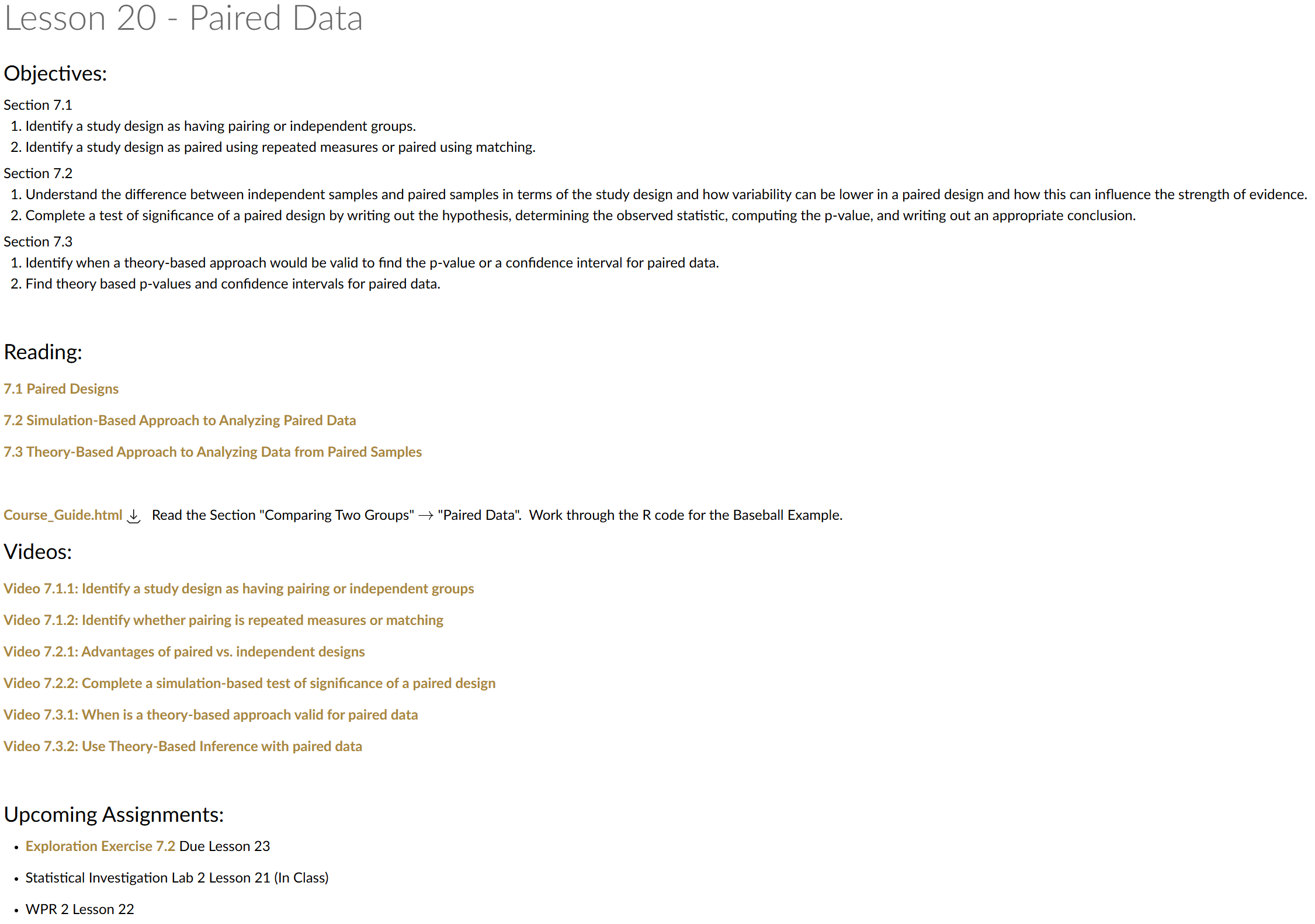
Lesson 20: Paired Data
Lesson Administration
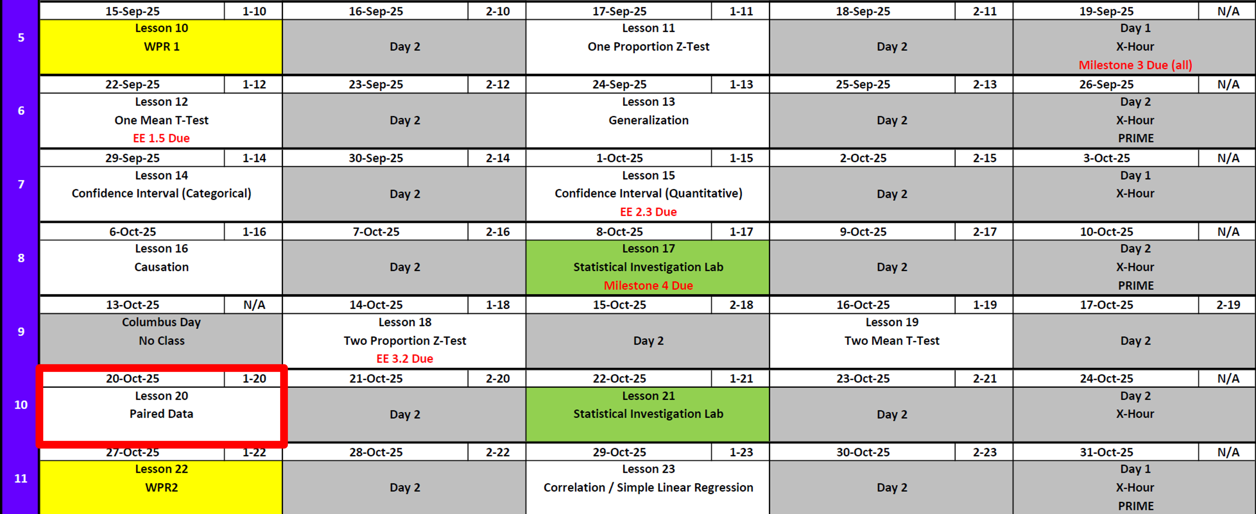
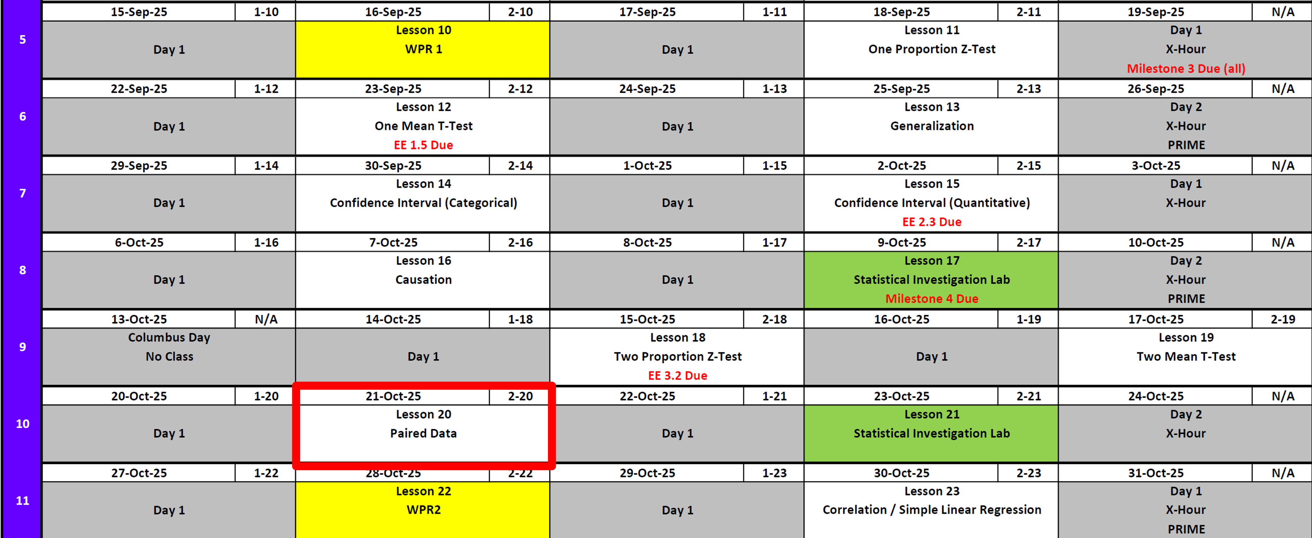
Calendar
Day 1
Day 2
SIL 1 (Next Class Review)
Exploration Exercise 3.2 (Grade This Class)
Lets go over the grading plan and solution and take about 10 minutes.
Exploration Exercise 7.2
EE7.2 due 0700 23 Oct
SIL 2
WPR 2
- Lesson 22
Milestone 5
- Due 0700 on 7 November
- Instructions
Cal

Running Review
Review: \(z\)-Tests for One Proportion
For all cases:
\(H_0:\ \pi = \pi_0\)
\[ z = \frac{\hat{p} - \pi_0}{\sqrt{\frac{\hat{p}\,(1-\hat{p})}{n}}} \]
| Alternative Hypothesis | Formula for \(p\)-value | R Code |
|---|---|---|
| \(H_A:\ \pi > \pi_0\) | \(p = 1 - \Phi(z)\) | p_val <- 1 - pnorm(z_stat) |
| \(H_A:\ \pi < \pi_0\) | \(p = \Phi(z)\) | p_val <- pnorm(z_stat) |
| \(H_A:\ \pi \neq \pi_0\) | \(p = 2 \cdot (1 - \Phi(|z|))\) | p_val <- 2 * (1 - pnorm(abs(z_stat))) |
Where:
- \(\hat{p} = R/n\) (sample proportion)
- \(\pi_0\) = hypothesized proportion under \(H_0\)
- \(\Phi(\cdot)\) = cumulative distribution function (CDF) of the standard normal distribution
Validity Conditions
- Number of successes and failures must be greater than 10.
Confidence Interval for \(\pi\) (one proportion)
\[ \hat{p} \;\pm\; z_{\,1-\alpha/2}\,\sqrt{\frac{\hat{p}\,(1-\hat{p})}{n}} \]
I am \((1 - \alpha)\%\) confident that the true population proportion \(\pi\) lies between \([\text{lower bound}, \text{upper bound}]\).
Review: \(t\)-Tests for One Mean
For all cases:
\(H_0:\ \mu = \mu_0\)
\[ t = \frac{\bar{x} - \mu_0}{s / \sqrt{n}} \]
| Alternative Hypothesis | Formula for \(p\)-value | R Code |
|---|---|---|
| \(H_A:\ \mu > \mu_0\) | \(p = 1 - F_{t,df}(t)\) | p_val <- 1 - pt(t_stat, df) |
| \(H_A:\ \mu < \mu_0\) | \(p = F_{t,df}(t)\) | p_val <- pt(t_stat, df) |
| \(H_A:\ \mu \neq \mu_0\) | \(p = 2 \cdot (1 - F_{t,df}(|t|))\) | p_val <- 2 * (1 - pt(abs(t_stat), df)) |
Where:
- \(\bar{x}\) = sample mean
- \(\mu_0\) = hypothesized mean under \(H_0\)
- \(s\) = sample standard deviation
- \(n\) = sample size
- \(df = n - 1\) (degrees of freedom)
- \(F_{t,df}(\cdot)\) = CDF of Student’s \(t\) distribution with \(df\) degrees of freedom
Validity Conditions
- Sample size must be greater than 30.
Confidence Interval for \(\mu\) (one mean)
\[ \bar{x} \;\pm\; t_{\,1-\alpha/2,\;df}\,\frac{s}{\sqrt{n}}, \qquad df = n-1 \] I am \((1 - \alpha)\%\) confident that the true population mean \((\mu)\) lies between \([\text{lower bound}, \text{upper bound}]\).
Review: \(z\)-Tests for Two Proportions
For all cases:
\(H_0:\ \pi_1 - \pi_2 = 0\)
\[ z \;=\; \frac{(\hat{p}_1 - \hat{p}_2) - (\pi_1 - \pi_2)}{\sqrt{\hat{p}(1-\hat{p})\left(\tfrac{1}{n_1} + \tfrac{1}{n_2}\right)}} \]
Where the pooled proportion is
\[ \hat{p} \;=\; \frac{x_1 + x_2}{n_1 + n_2}. \]
| Alternative Hypothesis | Formula for \(p\)-value | R Code |
|---|---|---|
| \(H_A:\ \pi_1 - \pi_2 > 0\) | \(p = 1 - \Phi(z)\) | p_val <- 1 - pnorm(z_stat) |
| \(H_A:\ \pi_1 - \pi_2 < 0\) | \(p = \Phi(z)\) | p_val <- pnorm(z_stat) |
| \(H_A:\ \pi_1 - \pi_2 \neq 0\) | \(p = 2 \cdot (1 - \Phi(|z|))\) | p_val <- 2 * (1 - pnorm(abs(z_stat))) |
Where:
- \(\hat{p}_1 = x_1/n_1\) (sample proportion in group 1)
- \(\hat{p}_2 = x_2/n_2\) (sample proportion in group 2)
- \(\pi_1, \pi_2\) = hypothesized proportions under \(H_0\)
- \(\Phi(\cdot)\) = cumulative distribution function (CDF) of the standard normal distribution
Validity Conditions
- Each group must have at least 10 successes and 10 failures.
Confidence Interval for \(\pi_1 - \pi_2\) (unpooled SE)
\[ (\hat{p}_1 - \hat{p}_2) \;\pm\; z_{\,1-\alpha/2}\, \sqrt{\tfrac{\hat{p}_1(1-\hat{p}_1)}{n_1} + \tfrac{\hat{p}_2(1-\hat{p}_2)}{n_2}} \]
I am \((1 - \alpha)\%\) confident that the true difference in population proportions \((\pi_1 - \pi_2)\) lies between \([\text{lower bound}, \text{upper bound}]\).
Review: \(t\)-Tests for Two Means
For all cases:
\(H_0:\ \mu_1 - \mu_2 = 0\)
\[ t = \frac{(\bar{x}_1 - \bar{x}_2) - 0}{\sqrt{\tfrac{s_1^2}{n_1} + \tfrac{s_2^2}{n_2}}} \]
| Alternative Hypothesis | Formula for \(p\)-value | R Code |
|---|---|---|
| \(H_A:\ \mu_1 - \mu_2 > 0\) | \(p = 1 - F_{t,df}(t)\) | p_val <- 1 - pt(t_stat, df) |
| \(H_A:\ \mu_1 - \mu_2 < 0\) | \(p = F_{t,df}(t)\) | p_val <- pt(t_stat, df) |
| \(H_A:\ \mu_1 - \mu_2 \neq 0\) | \(p = 2 \cdot (1 - F_{t,df}(|t|))\) | p_val <- 2 * (1 - pt(abs(t_stat), df)) |
Where:
- \(\bar{x}_1,\ \bar{x}_2\) = sample means in groups 1 and 2
- \(s_1,\ s_2\) = sample standard deviations
- \(n_1,\ n_2\) = sample sizes
- \(df = n_1 + n_2 - 2\)
- \(F_{t,df}(\cdot)\) = CDF of Student’s \(t\) distribution with \(df\) degrees of freedom
Validity Conditions
- Groups are independent
- Populations are approximately normal (or \(n_1, n_2\) large enough by CLT)
Confidence Interval for \(\mu_1 - \mu_2\)
\[ (\bar{x}_1 - \bar{x}_2) \;\pm\; t_{\,1-\alpha/2,\;df}\, \sqrt{\tfrac{s_1^2}{n_1} + \tfrac{s_2^2}{n_2}}, \qquad df = n_1+n_2-2 \]
I am \((1 - \alpha)\%\) confident that the true difference in population means \((\mu_1 - \mu_2)\) lies between \([\text{lower bound}, \text{upper bound}]\).
Interpreting the \(p\)-value
Rejecting \(H_0\)
> Since the \(p\)-value is less than \(\alpha\) (e.g., \(0.05\)), we reject the null hypothesis.
> We conclude that there is sufficient evidence to suggest that [state the alternative claim in context].Failing to Reject \(H_0\)
> Since the \(p\)-value is greater than \(\alpha\) (e.g., \(0.05\)), we fail to reject the null hypothesis.
> We conclude that there is not sufficient evidence to suggest that [state the alternative claim in context].Strength of evidence: Smaller \(p\) means stronger evidence against \(H_0\).
Other Notes
- Generalization: We can generalize results to a larger population if the data come from a random and representative sample of that population.
- Causation: We can claim causation if participants are randomly assigned to treatments in an experiment. Without random assignment, we can only conclude association, not causation.
\[ \begin{array}{|c|c|c|} \hline & \text{Randomly Sampled} & \text{Not Randomly Sampled} \\ \hline \textbf{Randomly Assigned} & \begin{array}{c} \text{Generalize: Yes} \\ \text{Causation: Yes} \end{array} & \begin{array}{c} \text{Generalize: No} \\ \text{Causation: Yes} \end{array} \\ \hline \textbf{Not Randomly Assigned} & \begin{array}{c} \text{Generalize: Yes} \\ \text{Causation: No} \end{array} & \begin{array}{c} \text{Generalize: No} \\ \text{Causation: No} \end{array} \\ \hline \end{array} \]
- Parameters vs. Statistics: A parameter is a fixed (but usually unknown) numerical value describing a population (e.g., \(\mu\), \(\sigma\), \(\pi\)). A statistic is a numerical value computed from a sample (e.g., \(\bar{x}\), \(s\), \(\hat{p}\)).
- Parameters = target (what we want to know).
- Statistics = evidence (what we can actually measure).
- We use statistics to estimate parameters, and because different samples give different statistics, we capture this variability with confidence intervals.
- Parameters = target (what we want to know).
| Quantity | Population (Parameter) | Sample (Statistic) |
|---|---|---|
| Center (mean) | \(\mu\) | \(\bar{x}\) |
| Spread (SD) | \(\sigma\) | \(s\) |
| Proportion “success” | \(\pi\) | \(\hat{p}\) |
Paired \(t\)-Test
Sometimes we do not have two independent groups, but instead two measurements on the same subjects (or matched pairs).
Examples:
- Before/after training scores
- Left vs. right leg strength in the same person
In these cases, we analyze the differences within pairs rather than treating them as two independent samples. This essentially becomes a one mean hypothesis test from before.
Example: Fitness Training
Researchers measured cadets’ mile times before and after a new training program. The same 22 cadets were tested twice.
| Cadet | Before | After |
|---|---|---|
| 1 | 7.20 | 7.80 |
| 2 | 6.95 | 7.60 |
| 3 | 7.40 | 8.10 |
| 4 | 7.00 | 6.70 |
| 5 | 6.85 | 6.60 |
| 6 | 7.25 | 7.00 |
| … | … | … |
We want to test if the program reduces mile time on average.
Step 1: Hypotheses
Let \(d = \text{Before – After}\).
- Null: \(H_0:\ \mu_d = 0\) (no change)
- Alternative: \(H_A:\ \mu_d > 0\) (before is greater than after \(\;\Rightarrow\;\) improved performance)
Step 2: Test Statistic
We compute a one-sample \(t\)-test on the differences:
\[ t \;=\; \frac{\bar{d} - 0}{s_d/\sqrt{n}}, \qquad df = n-1 \]
Step 3: Compute
\[ t = \frac{-0.143}{.325/\sqrt{22}} = \frac{-0.143}{0.067} \approx 2.06 \]
before <- c(7.20,6.95,7.40,7.00,6.85,7.25,7.05,6.90,7.10,6.80,7.00,6.95,7.15,7.05,7.20,6.85,7.30,7.00,6.95,7.10,7.05,7.25)

after <- c(7.80,7.60,8.10,6.70,6.60,7.00,6.90,6.55,6.85,6.50,6.70,6.65,6.85,6.80,6.95,6.60,7.00,6.75,6.70,6.85,6.80,6.95)

d <- before - after
n <- length(d)
dbar <- mean(d)
sd   <- sd(d)
df   <- n - 1

t_stat <- dbar / (sd/sqrt(n))
p_val  <- 1 - pt(t_stat, df)   # one-sided, "<" since After < Before

list(n = n, dbar = dbar, sd = sd, t_stat = t_stat, df = df, p_val = p_val)
$n
[1] 22
$dbar
[1] 0.1431818
$sd
[1] 0.3252455
$t_stat
[1] 2.064847
$df
[1] 21
$p_val
[1] 0.02575202Step 4: Decision
\(p \approx 0.026 < 0.05\)
\(\;\;\Rightarrow\) Reject \(H_0\).
We are 95% confident that the true mean difference in performance on mile time between the before and after is greater than 0.
Step 5: Confidence Interval
95% CI for \(\mu_d\):
\[ \bar{d} \;\pm\; t_{.025,\,df}\,\frac{s_d}{\sqrt{n}} \]
\[ = 0.143 \;\pm\; (2.08)(0.325) = 0.143\;\pm\; 0.144 = (-0.001,\; 0.287) \]
tcrit <- qt(0.025, df)

CI95 <- c(dbar + tcrit*(sd/sqrt(n)), dbar - tcrit*(sd/sqrt(n)))

list(dbar = dbar, sd = sd, df = df, tcrit = tcrit, CI95 = CI95)
$dbar
[1] 0.1431818
$sd
[1] 0.3252455
$df
[1] 21
$tcrit
[1] -2.079614
$CI95
[1] -0.001023956 0.287387592We are 95% confident that the training reduces mile time by -.001 to 0.287 minutes.
Yes, the CI includes 0. So in a \(\neq\) alternative hypothesis this would fail to reject.
Validity & Scope
- Validity: Differences are independent, approximately normal, and \(n=22\) is a reasonably large sample.
- Scope:
- If cadets were randomly sampled \(\;\Rightarrow\;\) generalize to population.
- If cadets were randomly assigned \(\;\Rightarrow\;\) can claim causation.
- If cadets were randomly sampled \(\;\Rightarrow\;\) generalize to population.
Board Problem: Does caffeine improve reaction time?
A group of cadets test whether drinking a small cup of coffee improves reaction time (measured in seconds). Each cadet is tested before and after drinking coffee.
- \(n=12\) cadets
- Mean difference (Before – After): \(\bar{d} = 0.18\) seconds
- Standard deviation of differences: \(s_d = 0.22\) seconds
Test, at \(\alpha=0.05\), whether coffee reduces average reaction time (i.e., improves performance). Also construct a 95% CI for \(\mu_d\).
- Define parameters and state hypotheses.
- Compute the test statistic, degrees of freedom, and one-sided \(p\)-value.
- Make a decision and interpret.
- Give the 95% CI and interpret it in context.
NoteSolution
Hypotheses
\(H_0:\ \mu_d = 0 \quad\text{vs}\quad H_A:\ \mu_d > 0\)
(where \(d =\) Before – After, so \(d>0\) means improvement)
Test statistic
\[ t = \frac{\bar{d} - 0}{s_d/\sqrt{n}} = \frac{0.18}{0.22/\sqrt{12}} = \frac{0.18}{0.064} \approx 2.81 \]
Degrees of freedom: \(df = n-1 = 11\)
One-sided \(p\)-value \(\approx 0.008\).
Decision: Reject \(H_0\).
Conclusion: There is strong evidence that coffee improves reaction time.
95% Confidence Interval
\[ \bar{d} \;\pm\; t_{0.975,\,df}\,\frac{s_d}{\sqrt{n}} = 0.18 \;\pm\; (2.20)(0.064) = 0.18 \;\pm\; 0.14 = (0.04,\; 0.32) \]
We are 95% confident that coffee reduces average reaction time by 0.04 to 0.32 seconds.
R code to verify
dbar <- 0.18; sd <- 0.22; n <- 12
df <- n - 1

t_stat <- dbar / (sd/sqrt(n))
p_val <- 1 - pt(t_stat, df)  # one-sided, "greater"

tcrit <- qt(0.975, df)
CI95 <- dbar + c(-1, 1) * tcrit * (sd/sqrt(n))

list(dbar = dbar, sd = sd, n = n, df = df,
     t_stat = t_stat, p_val = p_val,
     tcrit = tcrit, CI95 = CI95)
$dbar
[1] 0.18
$sd
[1] 0.22
$n
[1] 12
$df
[1] 11
$t_stat
[1] 2.834265
$p_val
[1] 0.008123858
$tcrit
[1] 2.200985
$CI95
[1] 0.04021867 0.31978133Before you leave
Today:
- Any questions for me?
Upcoming Graded Events
- WPR 2: Lesson 22