Lesson 25 - Multiple Linear Regression II
Lesson Administration
Calendar
Day 1

Day 2

SIL 2 Points
Milestone 5
- Lesson 25.5
- Change: 9 November 2359
- Milestone 5 Instructions
Exploration Exercise 4.4
- Lesson 26
- 12-13 November
- Link: TBD
Milestone 6: Draft Tech Report
- Lesson 26.5
- 17 November
- Milestone 6 Instructions
Project Presentations
- Need to know who will not be here on presentation day because of CPRC
Milestone 7
Milestone 8
TEE Times
| Date | Start | End |
|---|---|---|
| Wed, 17 Dec 2025 | 1300 | 1630 |
| Thu, 18 Dec 2025 | 0730 | 1100 |
DMath Basketball!!
Math 1 vs…
NotePreviously 0-0
1-0

Cal
Reese
I got nothing… So enjoy these
Multiple Linear Regression
A Reminder
Remember this from last class?
mod1 <- lm(formula = mpg ~ wt + as.factor(cyl), data = mtcars)
summary(mod1)
Call:
lm(formula = mpg ~ wt + as.factor(cyl), data = mtcars)

Residuals:
    Min      1Q  Median      3Q     Max
-4.5890 -1.2357 -0.5159  1.3845  5.7915

Coefficients:
                Estimate Std. Error t value Pr(>|t|)
(Intercept)      33.9908     1.8878  18.006  < 2e-16 ***
wt               -3.2056     0.7539  -4.252 0.000213 ***
as.factor(cyl)6  -4.2556     1.3861  -3.070 0.004718 **
as.factor(cyl)8  -6.0709     1.6523  -3.674 0.000999 ***
---
Signif. codes:  0 '***' 0.001 '**' 0.01 '*' 0.05 '.' 0.1 ' ' 1

Residual standard error: 2.557 on 28 degrees of freedom
Multiple R-squared:  0.8374,    Adjusted R-squared:   0.82
F-statistic: 48.08 on 3 and 28 DF,  p-value: 3.594e-11
The fitted regression equation is:
\[ \widehat{mpg} = 33.99 - 3.21(\text{wt}) - 4.26(\text{cyl6}) - 6.07(\text{cyl8}) \]
To predict fuel efficiency for a 3000-lb, 6-cylinder car:
\[ \begin{aligned} \widehat{mpg} &= 33.99 - 3.21(3.0) - 4.26(1) - 6.07(0) \\[6pt] &= 33.99 - 9.63 - 4.26 \\[6pt] &= 20.10 \end{aligned} \]
So the model predicts:
\[ \boxed{\widehat{mpg} = 20.1} \]
Interactions
mod2 <- lm(formula = mpg ~ wt + as.factor(cyl) + hp + hp:as.factor(cyl), data = mtcars)
summary(mod2)
Call:
lm(formula = mpg ~ wt + as.factor(cyl) + hp + hp:as.factor(cyl),
    data = mtcars)

Residuals:
    Min      1Q  Median      3Q     Max
-3.1864 -1.4098 -0.4022  1.0186  4.3920

Coefficients:
                    Estimate Std. Error t value Pr(>|t|)
(Intercept)         41.87732    3.23293  12.953 1.37e-12 ***
wt                  -3.05994    0.68275  -4.482 0.000143 ***
as.factor(cyl)6     -9.98213    5.76950  -1.730 0.095931 .
as.factor(cyl)8    -11.72793    4.22507  -2.776 0.010276 *
hp                  -0.09947    0.03487  -2.853 0.008576 **
as.factor(cyl)6:hp   0.07809    0.05236   1.492 0.148335
as.factor(cyl)8:hp   0.08602    0.03703   2.323 0.028601 *
---
Signif. codes:  0 '***' 0.001 '**' 0.01 '*' 0.05 '.' 0.1 ' ' 1

Residual standard error: 2.3 on 25 degrees of freedom
Multiple R-squared:  0.8826,    Adjusted R-squared:  0.8544
F-statistic: 31.32 on 6 and 25 DF,  p-value: 1.831e-10
We can write the fitted model as
\[ \begin{aligned} \widehat{mpg} &= 41.877 - 3.060\,(\text{wt}) - 9.982\,(\text{cyl6}) - 11.728\,(\text{cyl8}) - 0.09947\,(\text{hp}) + 0.07809\,(\text{hp}\times \text{cyl6}) + 0.08602\,(\text{hp}\times \text{cyl8}) \end{aligned} \]
Comparing Models
Which one is better?
Lets turn to \(R^2\)
Model 1: .8374
Model 2: .8826
Validity Conditions
Linearity — the relationship between predictors and the response is roughly linear
Independence — observations are independent of each other
Normal Distribution — residuals are approximately normal
Equal Variance — variability of residuals is consistent across fitted values
Linearity
Check whether the relationship between predictors and the response is roughly linear.
Use a residuals vs fitted plot — you want to see a random scatter (no pattern).
plot(mod1, which = 1)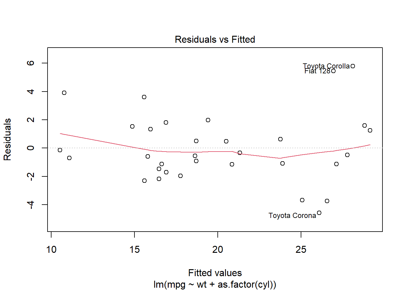
Independence
We can’t test this from the model alone — it depends on how the data were collected.
You must verify that each observation is independent (e.g., different cars, people, or trials).
Normal Distribution
Check whether residuals are approximately normally distributed using a Q-Q plot.
plot(mod1, which = 2)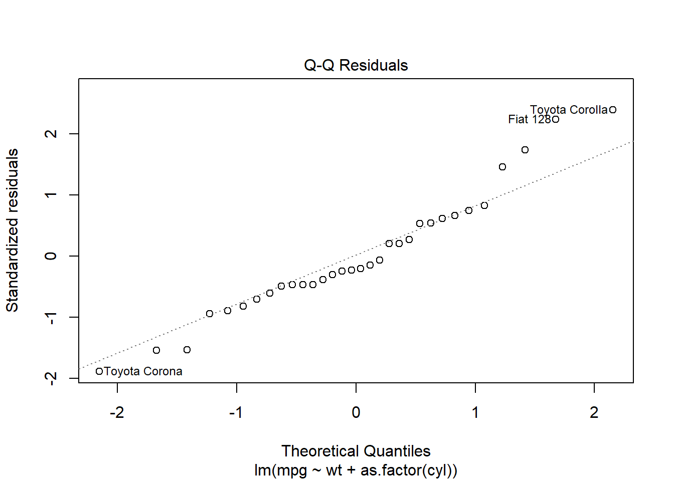
Equal Variance
Check for constant variance (homoscedasticity) — residuals should have similar spread across fitted values.
plot(mod1, which = 1)
Adventure One - Example of what to do for Milestone 5
library(tidyverse)

data("diamonds")

diamonds |>
  sample_n(size = 1000) |>
  pivot_longer(cols = -c(cut, clarity, price, color)) |>
  ggplot(aes(x = value, y = price, colour = color)) +
  geom_point() +
  facet_wrap(~name, scales = "free")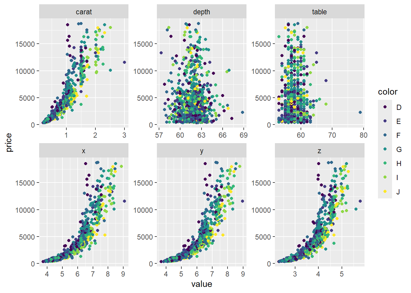
mod1 <- lm(formula = price ~ carat + depth + table + x + y + z + cut + color + clarity, data = diamonds)
summary(mod1)
Call:
lm(formula = price ~ carat + depth + table + x + y + z + cut +
    color + clarity, data = diamonds)

Residuals:
     Min       1Q   Median       3Q      Max
-21376.0   -592.4   -183.5    376.4  10694.2

Coefficients:
             Estimate Std. Error  t value Pr(>|t|)
(Intercept)  5753.762    396.630   14.507  < 2e-16 ***
carat       11256.978     48.628  231.494  < 2e-16 ***
depth         -63.806      4.535  -14.071  < 2e-16 ***
table         -26.474      2.912   -9.092  < 2e-16 ***
x           -1008.261     32.898  -30.648  < 2e-16 ***
y               9.609     19.333    0.497  0.61918
z             -50.119     33.486   -1.497  0.13448
cut.L         584.457     22.478   26.001  < 2e-16 ***
cut.Q        -301.908     17.994  -16.778  < 2e-16 ***
cut.C         148.035     15.483    9.561  < 2e-16 ***
cut^4         -20.794     12.377   -1.680  0.09294 .
color.L     -1952.160     17.342 -112.570  < 2e-16 ***
color.Q      -672.054     15.777  -42.597  < 2e-16 ***
color.C      -165.283     14.725  -11.225  < 2e-16 ***
color^4        38.195     13.527    2.824  0.00475 **
color^5       -95.793     12.776   -7.498 6.59e-14 ***
color^6       -48.466     11.614   -4.173 3.01e-05 ***
clarity.L    4097.431     30.259  135.414  < 2e-16 ***
clarity.Q   -1925.004     28.227  -68.197  < 2e-16 ***
clarity.C     982.205     24.152   40.668  < 2e-16 ***
clarity^4    -364.918     19.285  -18.922  < 2e-16 ***
clarity^5     233.563     15.752   14.828  < 2e-16 ***
clarity^6       6.883     13.715    0.502  0.61575
clarity^7      90.640     12.103    7.489 7.06e-14 ***
---
Signif. codes:  0 '***' 0.001 '**' 0.01 '*' 0.05 '.' 0.1 ' ' 1

Residual standard error: 1130 on 53916 degrees of freedom
Multiple R-squared:  0.9198,    Adjusted R-squared:  0.9198
F-statistic: 2.688e+04 on 23 and 53916 DF,  p-value: < 2.2e-16
mod2 <- lm(formula = price ~ carat + depth + table + x + z + cut + color + clarity, data = diamonds)
summary(mod2)
Call:
lm(formula = price ~ carat + depth + table + x + z + cut + color +
    clarity, data = diamonds)

Residuals:
     Min       1Q   Median       3Q      Max
-21378.8   -592.5   -183.5    376.3  10694.1

Coefficients:
             Estimate Std. Error  t value Pr(>|t|)
(Intercept)  5768.782    395.474   14.587  < 2e-16 ***
carat       11257.752     48.602  231.630  < 2e-16 ***
depth         -64.003      4.517  -14.168  < 2e-16 ***
table         -26.501      2.911   -9.103  < 2e-16 ***
x           -1000.354     28.795  -34.740  < 2e-16 ***
z             -47.925     33.194   -1.444  0.14880
cut.L         584.600     22.476   26.010  < 2e-16 ***
cut.Q        -302.211     17.983  -16.805  < 2e-16 ***
cut.C         148.446     15.461    9.601  < 2e-16 ***
cut^4         -20.619     12.371   -1.667  0.09559 .
color.L     -1952.179     17.342 -112.572  < 2e-16 ***
color.Q      -672.075     15.777  -42.599  < 2e-16 ***
color.C      -165.277     14.725  -11.224  < 2e-16 ***
color^4        38.193     13.526    2.824  0.00475 **
color^5       -95.780     12.776   -7.497 6.64e-14 ***
color^6       -48.452     11.614   -4.172 3.02e-05 ***
clarity.L    4097.613     30.256  135.431  < 2e-16 ***
clarity.Q   -1925.133     28.226  -68.205  < 2e-16 ***
clarity.C     982.322     24.150   40.676  < 2e-16 ***
clarity^4    -364.976     19.285  -18.926  < 2e-16 ***
clarity^5     233.635     15.751   14.833  < 2e-16 ***
clarity^6       6.871     13.715    0.501  0.61640
clarity^7      90.622     12.103    7.487 7.13e-14 ***
---
Signif. codes:  0 '***' 0.001 '**' 0.01 '*' 0.05 '.' 0.1 ' ' 1

Residual standard error: 1130 on 53917 degrees of freedom
Multiple R-squared:  0.9198,    Adjusted R-squared:  0.9198
F-statistic: 2.81e+04 on 22 and 53917 DF,  p-value: < 2.2e-16
## Candidate model
mod3 <- lm(formula = price ~ carat + depth + table + x + cut + color + clarity, data = diamonds)
summary(mod3)
Call:
lm(formula = price ~ carat + depth + table + x + cut + color +
    clarity, data = diamonds)

Residuals:
     Min       1Q   Median       3Q      Max
-21385.0   -592.4   -183.7    376.5  10694.6

Coefficients:
             Estimate Std. Error  t value Pr(>|t|)
(Intercept)  5935.107    378.328   15.688  < 2e-16 ***
carat       11256.968     48.600  231.626  < 2e-16 ***
depth         -66.769      4.091  -16.322  < 2e-16 ***
table         -26.457      2.911   -9.089  < 2e-16 ***
x           -1029.478     20.549  -50.098  < 2e-16 ***
cut.L         584.717     22.476   26.015  < 2e-16 ***
cut.Q        -302.037     17.983  -16.795  < 2e-16 ***
cut.C         148.065     15.459    9.578  < 2e-16 ***
cut^4         -21.253     12.364   -1.719  0.08562 .
color.L     -1952.128     17.342 -112.568  < 2e-16 ***
color.Q      -672.207     15.777  -42.608  < 2e-16 ***
color.C      -165.451     14.724  -11.236  < 2e-16 ***
color^4        38.261     13.526    2.829  0.00468 **
color^5       -95.816     12.776   -7.500 6.50e-14 ***
color^6       -48.441     11.614   -4.171 3.04e-05 ***
clarity.L    4096.912     30.253  135.423  < 2e-16 ***
clarity.Q   -1924.681     28.224  -68.192  < 2e-16 ***
clarity.C     982.004     24.149   40.664  < 2e-16 ***
clarity^4    -364.870     19.285  -18.920  < 2e-16 ***
clarity^5     233.449     15.751   14.822  < 2e-16 ***
clarity^6       6.973     13.715    0.508  0.61114
clarity^7      90.738     12.103    7.497 6.63e-14 ***
---
Signif. codes:  0 '***' 0.001 '**' 0.01 '*' 0.05 '.' 0.1 ' ' 1

Residual standard error: 1130 on 53918 degrees of freedom
Multiple R-squared:  0.9198,    Adjusted R-squared:  0.9198
F-statistic: 2.944e+04 on 21 and 53918 DF,  p-value: < 2.2e-16
diamonds |>
select(-c(cut, color, clarity)) |>
sample_n(1000) |>
pairs()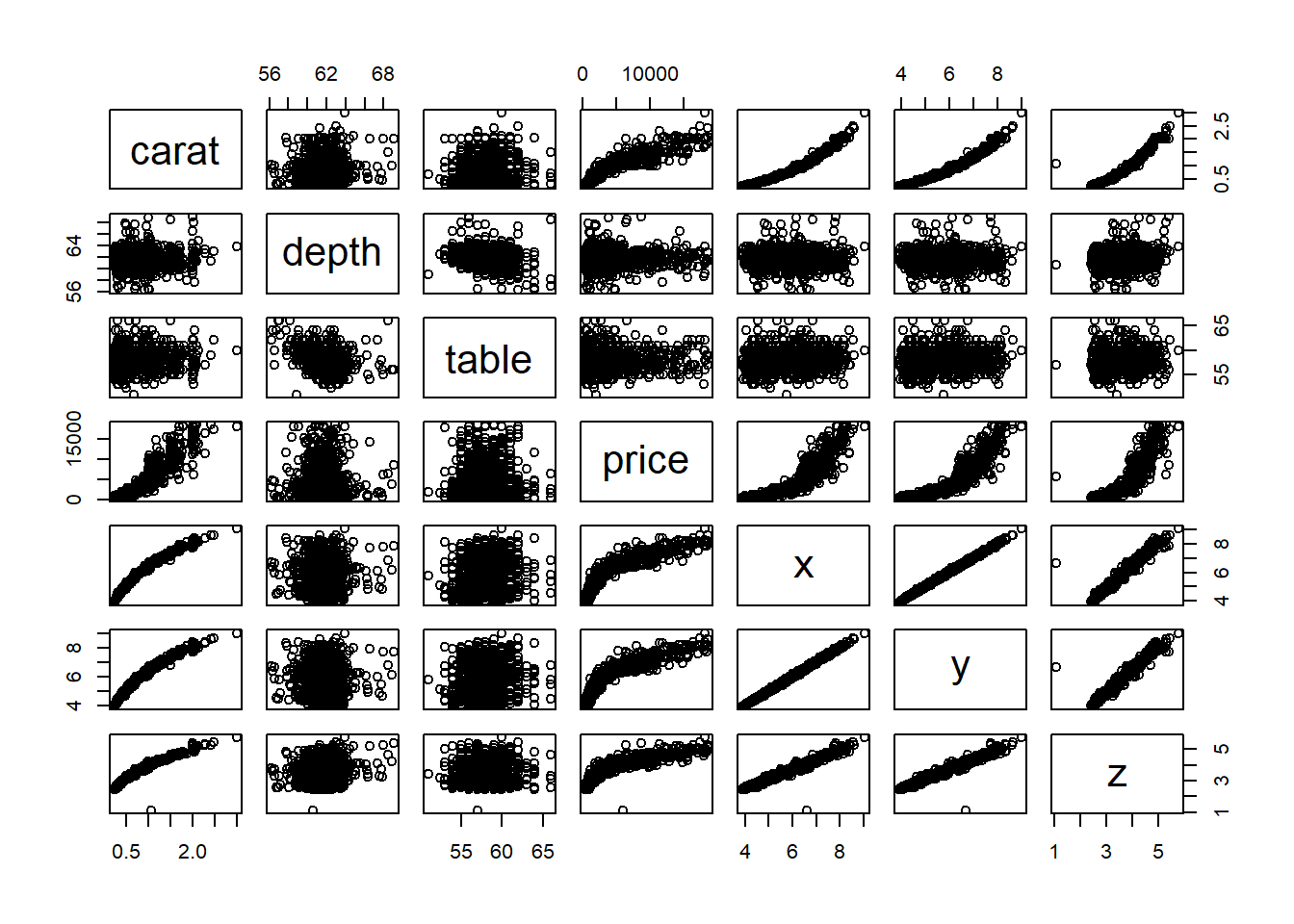
mod4 <- lm(formula = price ~ carat + depth + table + x + cut + color + clarity + carat:color, data = diamonds)
summary(mod4)
Call:
lm(formula = price ~ carat + depth + table + x + cut + color +
    clarity + carat:color, data = diamonds)

Residuals:
     Min       1Q   Median       3Q      Max
-16732.9   -513.8   -136.6    358.5  10550.5

Coefficients:
               Estimate Std. Error t value Pr(>|t|)
(Intercept)   10393.339    359.347  28.923  < 2e-16 ***
carat         12646.011     49.034 257.900  < 2e-16 ***
depth           -97.355      3.860 -25.223  < 2e-16 ***
table           -28.297      2.735 -10.348  < 2e-16 ***
x             -1624.864     20.623 -78.791  < 2e-16 ***
cut.L           594.594     21.114  28.161  < 2e-16 ***
cut.Q          -274.247     16.896 -16.232  < 2e-16 ***
cut.C           132.434     14.523   9.119  < 2e-16 ***
cut^4           -12.347     11.613  -1.063  0.28770
color.L         329.781     34.252   9.628  < 2e-16 ***
color.Q         513.842     31.643  16.239  < 2e-16 ***
color.C        -119.817     29.087  -4.119 3.81e-05 ***
color^4          69.759     26.171   2.665  0.00769 **
color^5         250.440     24.647  10.161  < 2e-16 ***
color^6         125.580     22.195   5.658 1.54e-08 ***
clarity.L      4113.880     28.459 144.556  < 2e-16 ***
clarity.Q     -1981.152     26.554 -74.607  < 2e-16 ***
clarity.C       991.093     22.698  43.665  < 2e-16 ***
clarity^4      -353.021     18.117 -19.485  < 2e-16 ***
clarity^5       208.673     14.801  14.099  < 2e-16 ***
clarity^6        26.858     12.884   2.085  0.03711 *
clarity^7       107.303     11.372   9.436  < 2e-16 ***
carat:color.L -2454.649     34.150 -71.878  < 2e-16 ***
carat:color.Q -1020.521     31.031 -32.887  < 2e-16 ***
carat:color.C   212.081     29.261   7.248 4.29e-13 ***
carat:color^4    19.164     27.152   0.706  0.48031
carat:color^5  -396.193     26.071 -15.196  < 2e-16 ***
carat:color^6  -192.062     24.204  -7.935 2.14e-15 ***
---
Signif. codes:  0 '***' 0.001 '**' 0.01 '*' 0.05 '.' 0.1 ' ' 1

Residual standard error: 1061 on 53912 degrees of freedom
Multiple R-squared:  0.9293,    Adjusted R-squared:  0.9292
F-statistic: 2.623e+04 on 27 and 53912 DF,  p-value: < 2.2e-16
## Candidate model
mod5 <- lm(formula = price ~ carat + depth + table + x + cut + color + clarity + carat:color + clarity:carat, data = diamonds)
summary(mod5)
Call:
lm(formula = price ~ carat + depth + table + x + cut + color +
    clarity + carat:color + clarity:carat, data = diamonds)

Residuals:
     Min       1Q   Median       3Q      Max
-22707.3   -301.6     -0.9    271.9   8784.4

Coefficients:
                 Estimate Std. Error  t value Pr(>|t|)
(Intercept)     21244.877    290.112   73.230  < 2e-16 ***
carat           16453.723     45.710  359.960  < 2e-16 ***
depth            -163.331      3.068  -53.232  < 2e-16 ***
table             -39.541      2.158  -18.324  < 2e-16 ***
x               -3095.798     18.360 -168.620  < 2e-16 ***
cut.L             514.155     16.659   30.863  < 2e-16 ***
cut.Q            -163.316     13.343  -12.239  < 2e-16 ***
cut.C              71.287     11.459    6.221 4.98e-10 ***
cut^4               7.700      9.160    0.841  0.40059
color.L           667.031     27.200   24.523  < 2e-16 ***
color.Q           367.411     25.005   14.694  < 2e-16 ***
color.C            15.497     22.987    0.674  0.50022
color^4           104.494     20.654    5.059 4.22e-07 ***
color^5           200.370     19.445   10.305  < 2e-16 ***
color^6            24.333     17.523    1.389  0.16495
clarity.L       -3011.134     48.745  -61.774  < 2e-16 ***
clarity.Q        1767.264     44.991   39.280  < 2e-16 ***
clarity.C       -1411.691     37.984  -37.166  < 2e-16 ***
clarity^4         863.630     30.089   28.703  < 2e-16 ***
clarity^5        -454.165     24.029  -18.901  < 2e-16 ***
clarity^6         112.514     20.512    5.485 4.15e-08 ***
clarity^7         -91.019     17.879   -5.091 3.58e-07 ***
carat:color.L   -2936.145     27.224 -107.853  < 2e-16 ***
carat:color.Q    -861.382     24.531  -35.114  < 2e-16 ***
carat:color.C      33.212     23.141    1.435  0.15124
carat:color^4     -64.953     21.442   -3.029  0.00245 **
carat:color^5    -293.108     20.575  -14.246  < 2e-16 ***
carat:color^6     -24.459     19.136   -1.278  0.20119
carat:clarity.L  7881.781     51.240  153.820  < 2e-16 ***
carat:clarity.Q -2165.582     45.783  -47.301  < 2e-16 ***
carat:clarity.C  1714.611     41.112   41.706  < 2e-16 ***
carat:clarity^4  -945.245     36.053  -26.218  < 2e-16 ***
carat:clarity^5   488.264     31.404   15.548  < 2e-16 ***
carat:clarity^6    28.838     27.156    1.062  0.28827
carat:clarity^7   279.667     21.976   12.726  < 2e-16 ***
---
Signif. codes:  0 '***' 0.001 '**' 0.01 '*' 0.05 '.' 0.1 ' ' 1

Residual standard error: 837 on 53905 degrees of freedom
Multiple R-squared:  0.956, Adjusted R-squared:  0.956
F-statistic: 3.445e+04 on 34 and 53905 DF,  p-value: < 2.2e-16
#Linear
plot(mod5, which = 1)
#Inedpendence

# N
plot(mod5, which = 2)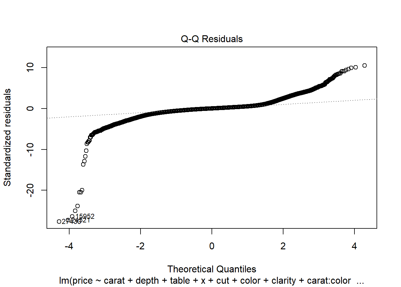
#E
plot(mod5, which = 1)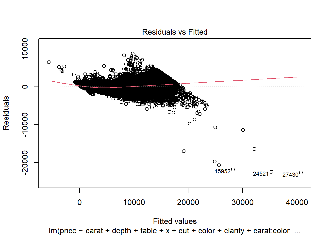
In Class Exercise - Adventure Two - Will revisit lesson 26
library(tidyverse)
diamonds
# A tibble: 53,940 × 10
carat cut color clarity depth table price x y z
<dbl> <ord> <ord> <ord> <dbl> <dbl> <int> <dbl> <dbl> <dbl>
1 0.23 Ideal E SI2 61.5 55 326 3.95 3.98 2.43
2 0.21 Premium E SI1 59.8 61 326 3.89 3.84 2.31
3 0.23 Good E VS1 56.9 65 327 4.05 4.07 2.31
4 0.29 Premium I VS2 62.4 58 334 4.2 4.23 2.63
5 0.31 Good J SI2 63.3 58 335 4.34 4.35 2.75
6 0.24 Very Good J VVS2 62.8 57 336 3.94 3.96 2.48
7 0.24 Very Good I VVS1 62.3 57 336 3.95 3.98 2.47
8 0.26 Very Good H SI1 61.9 55 337 4.07 4.11 2.53
9 0.22 Fair E VS2 65.1 61 337 3.87 3.78 2.49
10 0.23 Very Good H VS1 59.4 61 338 4 4.05 2.39
# ℹ 53,930 more rowsIn addition to carat size, what other variables might be associated with the price of a diamond?
Create a comparative box plot of
price(response variable on the y-axis) bycut(explanatory variable on the x-axis).
Which cut category tends to have higher prices? Is this what you would expect?Fit a simple linear model for
priceusingcaratas the explanatory variable andpriceas the response variable.
- Write out the regression equation with intercept, coefficients, and variable names.
- Interpret the coefficient of
caratin the context of this model.
- What is the strength of evidence that
caratis related toprice?
Create a scatterplot of
priceversuscarat, colored bycut.
Do higher-quality cuts tend to cluster at different price or carat ranges?
How might this influence your interpretation of the relationship between carat and price?Fit a multiple regression model for
priceusing bothcaratandcutas explanatory variables.
- Write out the regression equation with intercept, coefficients, and variable names.
- Interpret the coefficient for
cutwhile controlling forcarat.
How much total variation in diamond price is explained by this model (i.e., (R^2))?
The model in #5 assumes that the effect of
caratonpriceis the same across all cuts.
How can we check whether this assumption is valid?Fit a multiple regression model for
priceusing bothcaratandcut, including an interaction between them.
Write out the regression equation with intercept, coefficients, and variable names.Among the Ideal cut diamonds, how much does price increase for a one-unit increase in carat?
Among the Fair cut diamonds, how much does price increase for a one-unit increase in carat?
Is the interaction between
caratandcutstatistically significant?
State your null and alternative hypotheses for the interaction term and report the test statistic and p-value.To what population are you willing to generalize your results?
Can you draw a cause-and-effect conclusion about carat size and diamond price? Why or why not?
Partial Solution
Ask a Research Question
- In addition to carat size, what other variables might be associated with the price of a diamond?
Design a Study and Explore the Data
The diamonds dataset in R contains information about 53,940 diamonds, including their price (in U.S. dollars), carat, cut, color, clarity, and several physical measurements (x, y, z, depth, table).
We’ll examine how carat size and quality characteristics relate to diamond price.
- Use R to create a comparative box plot of
price(Response Variable on the y-axis) bycut(Explanatory Variable on the x-axis).- Which cut category tends to have higher prices?
- Is this what you would expect?
- Which cut category tends to have higher prices?
ggplot(diamonds, aes(x = cut, y = price)) +
  geom_boxplot() +
  labs(title = "Diamond Price by Cut Quality")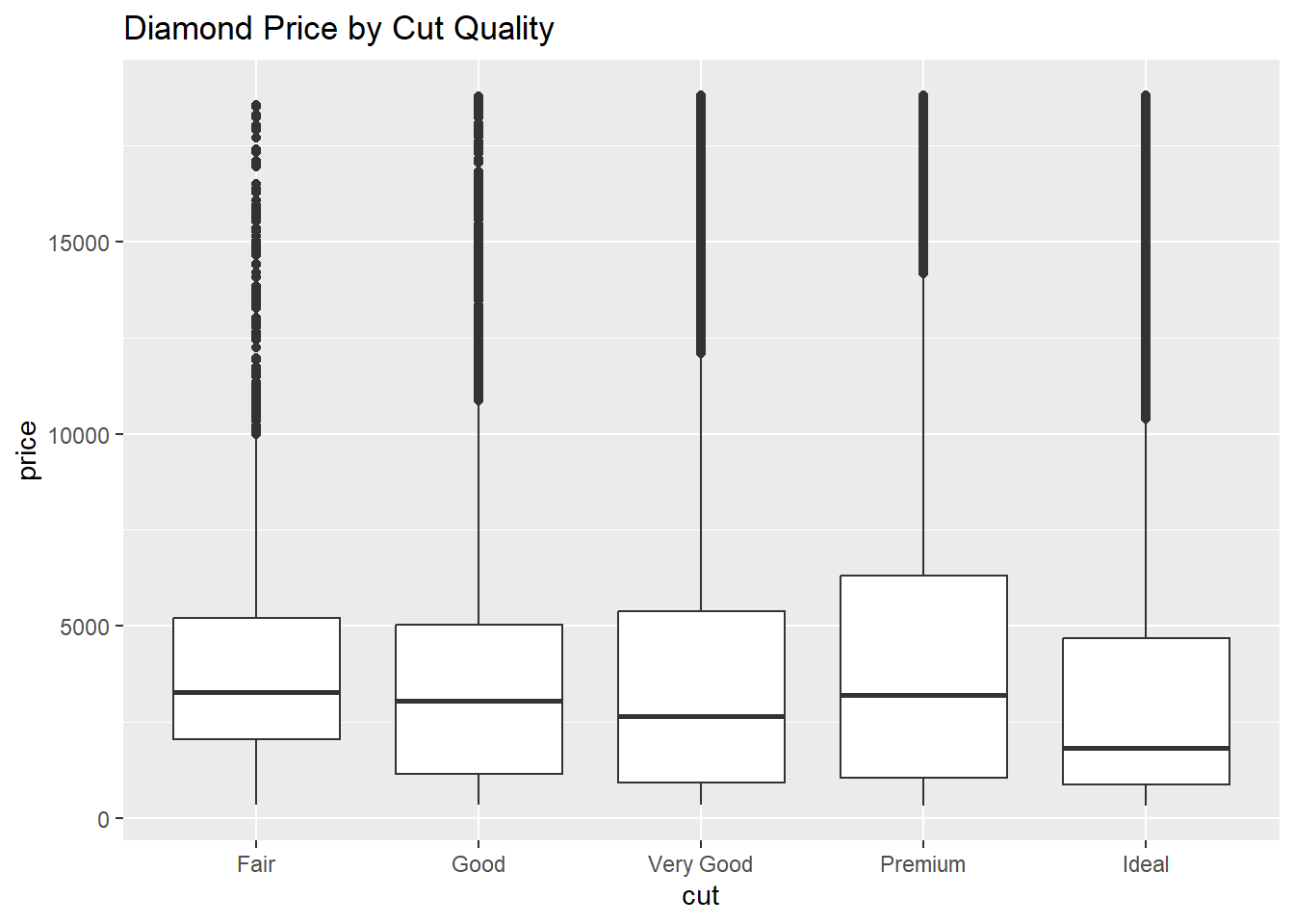
- Create a simple linear model for
priceusingcaratas the Explanatory Variable andpriceas the Response Variable.
mod1 <- lm(price ~ carat, data = diamonds)
summary(mod1)
Call:
lm(formula = price ~ carat, data = diamonds)

Residuals:
     Min       1Q   Median       3Q      Max
-18585.3   -804.8    -18.9    537.4  12731.7

Coefficients:
            Estimate Std. Error t value Pr(>|t|)
(Intercept) -2256.36      13.06  -172.8   <2e-16 ***
carat        7756.43      14.07   551.4   <2e-16 ***
---
Signif. codes:  0 '***' 0.001 '**' 0.01 '*' 0.05 '.' 0.1 ' ' 1

Residual standard error: 1549 on 53938 degrees of freedom
Multiple R-squared:  0.8493,    Adjusted R-squared:  0.8493
F-statistic: 3.041e+05 on 1 and 53938 DF, p-value: < 2.2e-16- Write out the simple linear regression equation with intercept, coefficients, and variable names.
\[ \widehat{price} = b_0 + b_1(\text{carat}) \]
- Interpret the coefficient of carat in the context of this model.
- Based on the p-value for the slope, what is the strength of evidence that
caratis related toprice?
- Generate a scatterplot of
price(y-axis) versuscarat(x-axis), colored bycut.
ggplot(diamonds, aes(x = carat, y = price, color = cut)) +
  geom_point(alpha = 0.5) +
  labs(title = "Diamond Price vs. Carat, by Cut")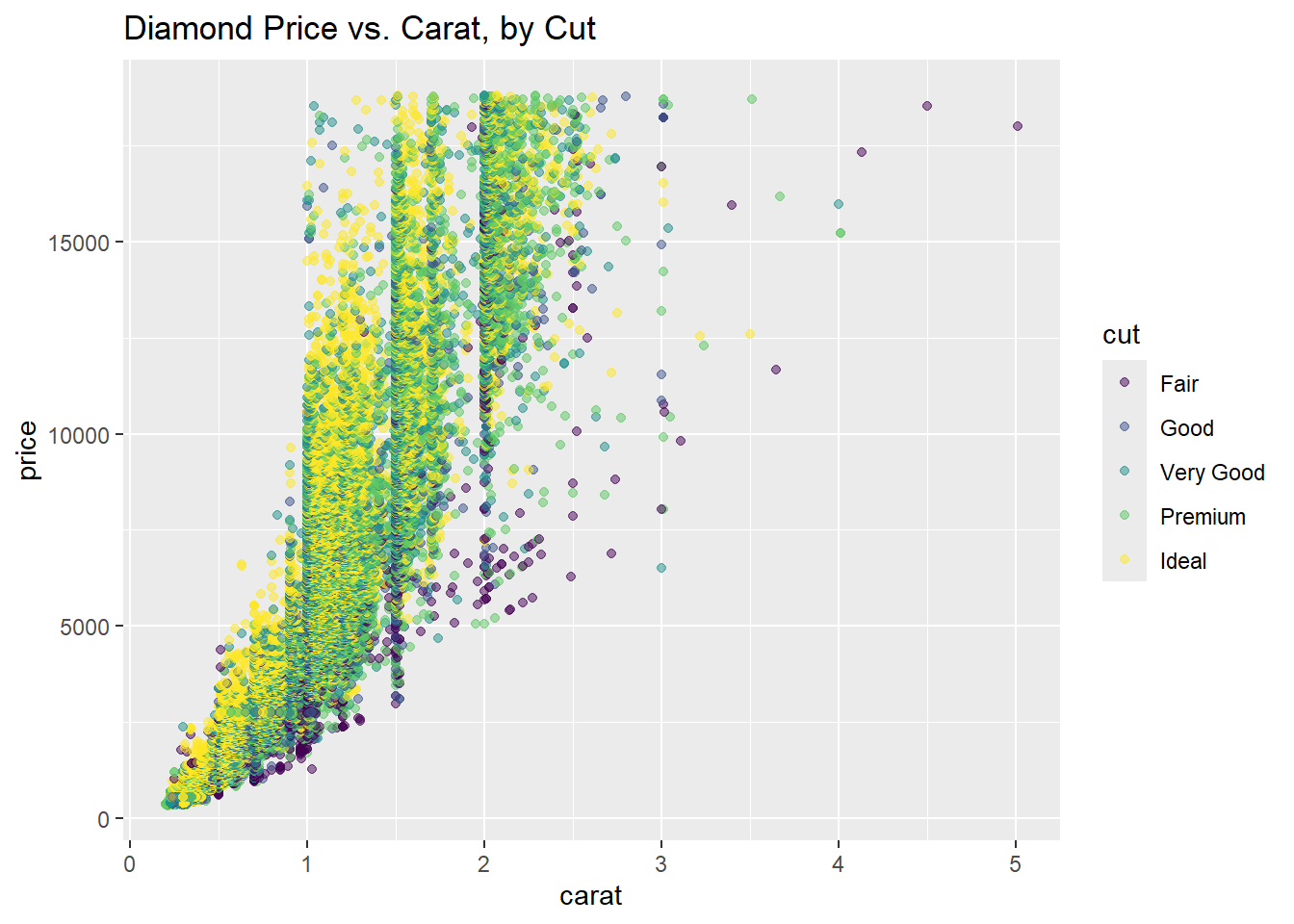
- Do higher-quality cuts tend to cluster at different price or carat ranges?
- How might this influence your interpretation of the relationship between carat and price?
- Fit a multiple regression model for
priceusing bothcaratandcutas Explanatory Variables.
mod2 <- lm(price ~ carat + cut, data = diamonds)
summary(mod2)
Call:
lm(formula = price ~ carat + cut, data = diamonds)

Residuals:
     Min       1Q   Median       3Q      Max
-17540.7   -791.6    -37.6    522.1  12721.4

Coefficients:
            Estimate Std. Error  t value Pr(>|t|)
(Intercept) -2701.38      15.43 -175.061  < 2e-16 ***
carat        7871.08      13.98  563.040  < 2e-16 ***
cut.L        1239.80      26.10   47.502  < 2e-16 ***
cut.Q        -528.60      23.13  -22.851  < 2e-16 ***
cut.C         367.91      20.21   18.201  < 2e-16 ***
cut^4          74.59      16.24    4.593 4.37e-06 ***
---
Signif. codes:  0 '***' 0.001 '**' 0.01 '*' 0.05 '.' 0.1 ' ' 1

Residual standard error: 1511 on 53934 degrees of freedom
Multiple R-squared:  0.8565,    Adjusted R-squared:  0.8565
F-statistic: 6.437e+04 on 5 and 53934 DF, p-value: < 2.2e-16- Write out the multiple regression equation with intercept, coefficients, and variable names.
- Interpret the coefficient for
cutwhile controlling forcarat.
How much total variation in diamond price is explained by this model (i.e., (R^2))?
This model assumes that the effect of carat on price is the same across all cuts.
- How can we check whether this assumption is valid?
Create a multiple regression model for
priceusing bothcaratandcut, including an interaction between them.
mod3 <- lm(price ~ carat * cut, data = diamonds)
summary(mod3)
Call:
lm(formula = price ~ carat * cut, data = diamonds)

Residuals:
     Min       1Q   Median       3Q      Max
-14878.3   -793.0    -23.0    546.3  12706.2

Coefficients:
            Estimate Std. Error  t value Pr(>|t|)
(Intercept) -2271.95      20.94 -108.513  < 2e-16 ***
carat        7468.05      19.49  383.200  < 2e-16 ***
cut.L        -278.21      57.17   -4.866 1.14e-06 ***
cut.Q         363.22      50.51    7.191 6.50e-13 ***
cut.C        -172.96      42.81   -4.041 5.34e-05 ***
cut^4          67.55      33.40    2.022   0.0431 *
carat:cut.L  1538.10      50.96   30.183  < 2e-16 ***
carat:cut.Q  -781.89      45.89  -17.037  < 2e-16 ***
carat:cut.C   509.65      41.36   12.321  < 2e-16 ***
carat:cut^4    69.70      34.38    2.027   0.0426 *
---
Signif. codes:  0 '***' 0.001 '**' 0.01 '*' 0.05 '.' 0.1 ' ' 1

Residual standard error: 1498 on 53930 degrees of freedom
Multiple R-squared:  0.8591,    Adjusted R-squared:  0.859
F-statistic: 3.653e+04 on 9 and 53930 DF,  p-value: < 2.2e-16
Write out the regression equation with intercept, coefficients, and variable names.
\[ \widehat{price} = b_0 + b_1(\text{carat}) + b_2(\text{cut}) + b_3(\text{carat} \times \text{cut}) \]
Among the Ideal cut diamonds, how much does price increase for a one-unit increase in carat?
Among the Fair cut diamonds, how much does price increase for a one-unit increase in carat?
Is the interaction between
caratandcutstatistically significant?- State your null and alternative hypotheses for the interaction term.
- Report the test statistic and p-value.
- State your null and alternative hypotheses for the interaction term.
To what population are you willing to generalize your results?
- Can you draw a cause-and-effect conclusion about carat size and diamond price?
- Why or why not?
- Can you draw a cause-and-effect conclusion about carat size and diamond price?
Check each of the four Validity Conditions for the multiple regression you ran in #8.
- Include all three validity plots for your regression model.
- Justify each of the four conditions: Linearity, Independence, Normality, and Equal Variance.
- Include all three validity plots for your regression model.
Linearity
plot(mod3, which = 1)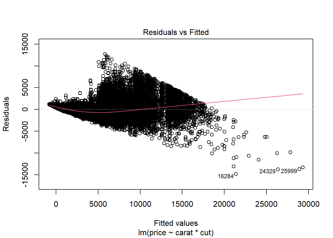
Independence
Must be justified based on data collection (not tested statistically).
Normal Distribution
plot(mod3, which = 2)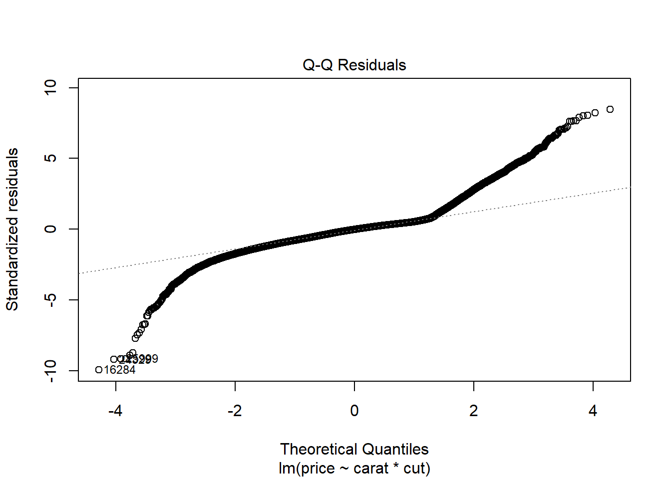
Equal Variance
plot(mod3, which = 1)
Before you leave
Today:
- Any questions for me?