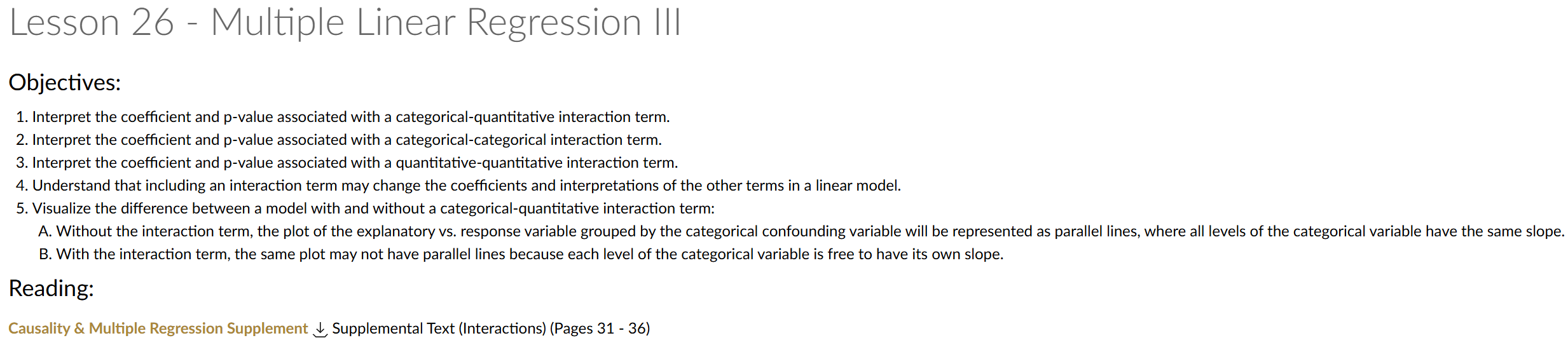
Lesson 26 - Multiple Linear Regression III
Lesson Administration
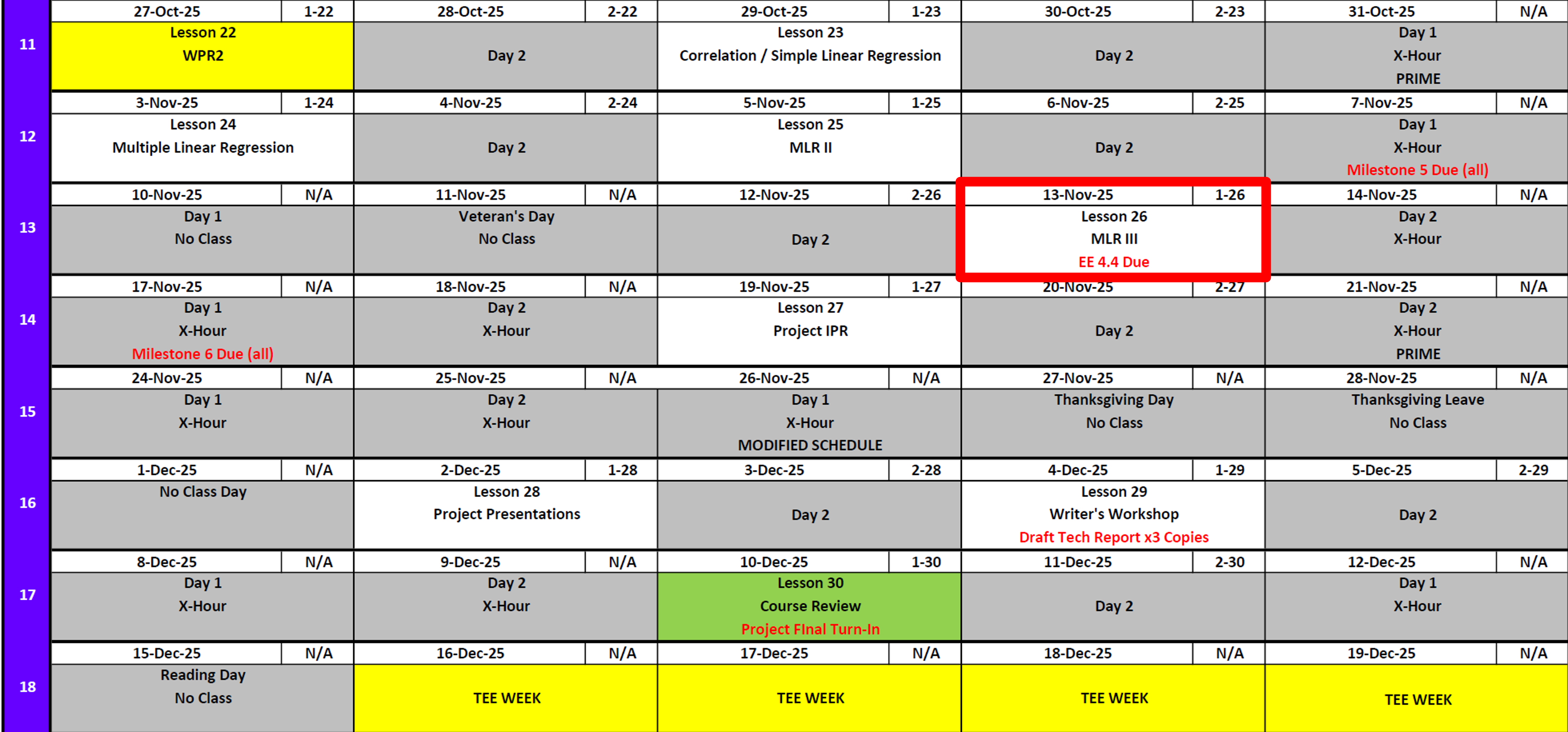
Calendar
Day 1
Day 2

No GradeScope
Download your feedback from GradeScope.
Exploration Exercise 4.4
- Lesson 26
- 12-13 November 2025
- Link: EE 4.4
Milestone 6: Draft Tech Report
- Lesson 26.5
- 17 November
- Milestone 6 Instructions
IPR
- Lesson 27
- Draft Presentation
- Presentation Template
Project Presentations
- Need to know who will not be here on presentation day because of CPRC
- 2/3 December - Primary
- 24/25 Nov Alternate
My current expectations
NoteG1
2 Dec
- 1: Charles Goetz, John McKillop
- 2: Jack McDaniel, Hunter McDonnell
- 4: Jenna Din, Karina Lawrence
- 5: John Afari-Aikins, Joshua George
- 6: Harrison Lavery, James Midberry, Macoy Noack
- 7: Nathan Coldren, Aarav Gupta
- 8: Brandon Freeman, John Minicozzi
24 Nov - 3: Annabella Conti, Tehya Meers
NoteH1
2 Dec
- 1: Joseph Johnson, Nehemiah Vann
- 2: Lucas Kinkead, Andrew Rubio
- 3: Cherokee Chambers, Trevor Thanepohn
- 4: Mary Arengo, Chad Dohl
- 5: Vanessa Hudson-Odoi, Tatiana Stockbower
- 6: Sawyer Shelton, Benjamin Walter
- 9: Campbell Sager, Samuel Zagame
24 Nov
- 7: Liam Wills, Logan Wint
- 8: Paul Chau, Benjamin Records
NoteI1
2 Dec
- 1: Elena Andrade, Gabrielle Warnre
- 2: Evan Campbell, Allan Sindler
- 3: Benjamin Aguilar Winchell, Dillon Bhutani
- 4: Bahawal Maan, Joseph Schwartz
- 5: Jacob Bettencourt, Daniel Ogordi
- 6: Braeden Helmkamp, Isabela Tahmazian
- 7: Barbara Forgues, Alex Jo
- 8: David Ahn, Sangwoo Park
- 9: Gennaro Smith
24 Nov
- 9: Logan Lanham
NoteI2
3 Dec
25 Nov
Paige McPherson Justin Davidson
Christian Bachmann Parker Harris
Milestone 7
- Draft Technical Report
- Lesson 29: Bring 3 Copies
Milestone 8
- Final Technical Report
- Course Review
TEE Times
| Date | Start | End |
|---|---|---|
| Wed, 17 Dec 2025 | 1300 | 1630 |
| Thu, 18 Dec 2025 | 0730 | 1100 |
DMath Frisbee PLAYOFFS!!
Math 1 vs Systems and Friends
NotePreviously 7-0
8-0

Army
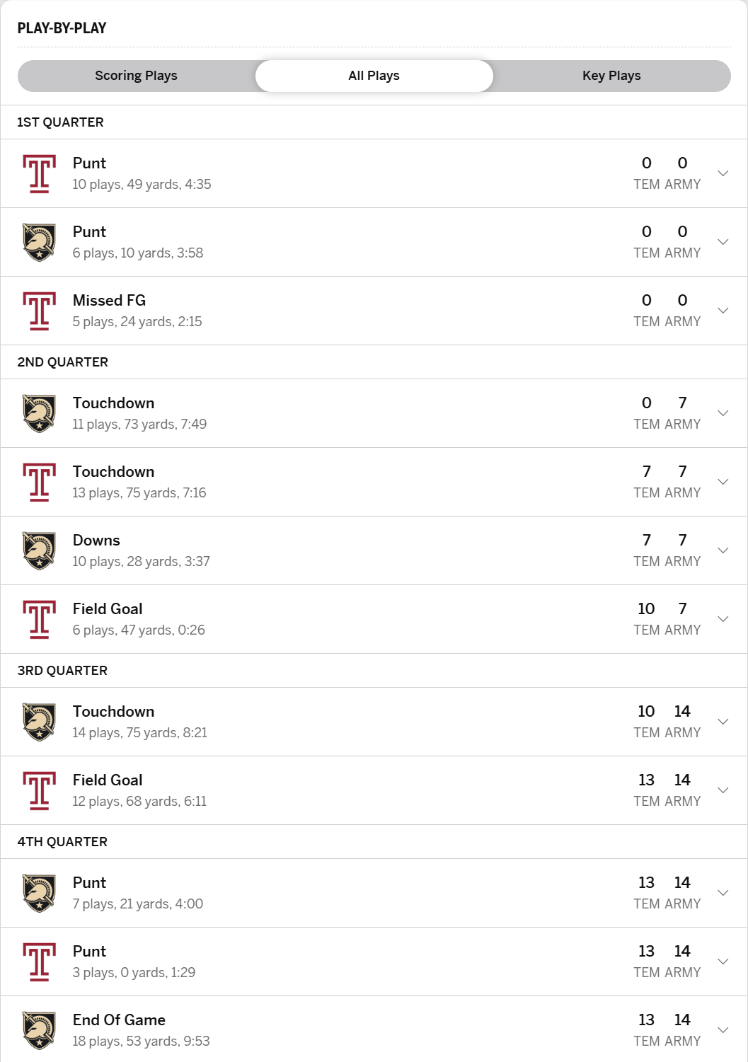
Reese
Me
Multiple Linear Regression
A Reminder
mod1 <- lm(formula = mpg ~ wt + as.factor(cyl) + hp + hp:as.factor(cyl), data = mtcars)
summary(mod1)
Call:
lm(formula = mpg ~ wt + as.factor(cyl) + hp + hp:as.factor(cyl),
    data = mtcars)

Residuals:
    Min      1Q  Median      3Q     Max
-3.1864 -1.4098 -0.4022  1.0186  4.3920

Coefficients:
                    Estimate Std. Error t value Pr(>|t|)
(Intercept)         41.87732    3.23293  12.953 1.37e-12 ***
wt                  -3.05994    0.68275  -4.482 0.000143 ***
as.factor(cyl)6     -9.98213    5.76950  -1.730 0.095931 .
as.factor(cyl)8    -11.72793    4.22507  -2.776 0.010276 *
hp                  -0.09947    0.03487  -2.853 0.008576 **
as.factor(cyl)6:hp   0.07809    0.05236   1.492 0.148335
as.factor(cyl)8:hp   0.08602    0.03703   2.323 0.028601 *
---
Signif. codes:  0 '***' 0.001 '**' 0.01 '*' 0.05 '.' 0.1 ' ' 1

Residual standard error: 2.3 on 25 degrees of freedom
Multiple R-squared:  0.8826,    Adjusted R-squared:  0.8544
F-statistic: 31.32 on 6 and 25 DF,  p-value: 1.831e-10
We can write the fitted model as
\[ \begin{aligned} \widehat{mpg} &= 41.877 - 3.060\,(\text{wt}) - 9.982\,(\text{cyl6}) - 11.728\,(\text{cyl8}) - 0.09947\,(\text{hp}) + 0.07809\,(\text{hp}\times \text{cyl6}) + 0.08602\,(\text{hp}\times \text{cyl8}) \end{aligned} \]
Linearity — the relationship between predictors and the response is roughly linear
Independence — observations are independent of each other
Normal Distribution — residuals are approximately normal
Equal Variance — variability of residuals is consistent across fitted values
Linearity
Check whether the relationship between predictors and the response is roughly linear.
Use a residuals vs fitted plot — you want to see a random scatter (no pattern).
plot(mod1, which = 1)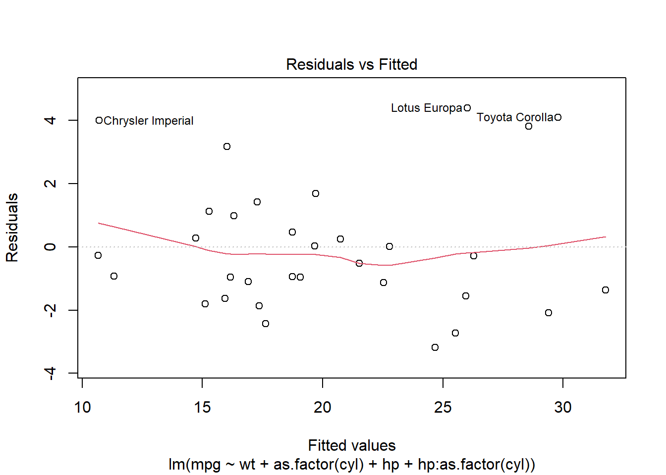
Independence
We can’t test this from the model alone — it depends on how the data were collected.
You must verify that each observation is independent (e.g., different cars, people, or trials).
Normal Distribution
Check whether residuals are approximately normally distributed using a Q-Q plot.
plot(mod1, which = 2)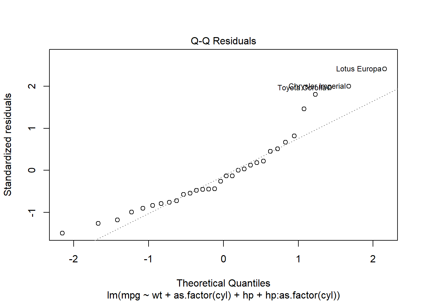
Equal Variance
Check for constant variance (homoscedasticity) — residuals should have similar spread across fitted values.
plot(mod1, which = 1)
In Class Exercise
library(tidyverse)
diamonds
# A tibble: 53,940 × 10
carat cut color clarity depth table price x y z
<dbl> <ord> <ord> <ord> <dbl> <dbl> <int> <dbl> <dbl> <dbl>
1 0.23 Ideal E SI2 61.5 55 326 3.95 3.98 2.43
2 0.21 Premium E SI1 59.8 61 326 3.89 3.84 2.31
3 0.23 Good E VS1 56.9 65 327 4.05 4.07 2.31
4 0.29 Premium I VS2 62.4 58 334 4.2 4.23 2.63
5 0.31 Good J SI2 63.3 58 335 4.34 4.35 2.75
6 0.24 Very Good J VVS2 62.8 57 336 3.94 3.96 2.48
7 0.24 Very Good I VVS1 62.3 57 336 3.95 3.98 2.47
8 0.26 Very Good H SI1 61.9 55 337 4.07 4.11 2.53
9 0.22 Fair E VS2 65.1 61 337 3.87 3.78 2.49
10 0.23 Very Good H VS1 59.4 61 338 4 4.05 2.39
# ℹ 53,930 more rowsIn addition to carat size, what other variables might be associated with the price of a diamond?
Create a comparative box plot of
price(response variable on the y-axis) bycut(explanatory variable on the x-axis).
Which cut category tends to have higher prices? Is this what you would expect?Fit a simple linear model for
priceusingcaratas the explanatory variable andpriceas the response variable.
- Write out the regression equation with intercept, coefficients, and variable names.
- Interpret the coefficient of
caratin the context of this model.
- What is the strength of evidence that
caratis related toprice?
Create a scatterplot of
priceversuscarat, colored bycut.
Do higher-quality cuts tend to cluster at different price or carat ranges?
How might this influence your interpretation of the relationship between carat and price?Fit a multiple regression model for
priceusing bothcaratandcutas explanatory variables.
- Write out the regression equation with intercept, coefficients, and variable names.
- Interpret the coefficient for
cutwhile controlling forcarat.
How much total variation in diamond price is explained by this model (i.e., (R^2))?
Fit a multiple regression model for
priceusing bothcaratandcut, including an interaction between them.
Write out the regression equation with intercept, coefficients, and variable names.Among the Ideal cut diamonds, how much does price increase for a one-unit increase in carat?
Among the Fair cut diamonds, how much does price increase for a one-unit increase in carat?
Is the interaction between
caratandcutstatistically significant?
State your null and alternative hypotheses for the interaction term and report the test statistic and p-value.To what population are you willing to generalize your results?
Can you draw a cause-and-effect conclusion about carat size and diamond price? Why or why not?Check each of the four Validity Conditions for the Multiple Regression you conducted in #7.
Partial Solution
Ask a Research Question
- In addition to carat size, what other variables might be associated with the price of a diamond?
Design a Study and Explore the Data
The diamonds dataset in R contains information about 53,940 diamonds, including their price (in U.S. dollars), carat, cut, color, clarity, and several physical measurements (x, y, z, depth, table).
We’ll examine how carat size and quality characteristics relate to diamond price.
- Use R to create a comparative box plot of
price(Response Variable on the y-axis) bycut(Explanatory Variable on the x-axis).- Which cut category tends to have higher prices?
- Is this what you would expect?
- Which cut category tends to have higher prices?
ggplot(diamonds, aes(x = cut, y = price)) +
  geom_boxplot() +
  labs(title = "Diamond Price by Cut Quality")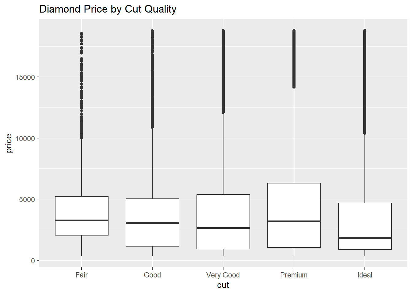
- Create a simple linear model for
priceusingcaratas the Explanatory Variable andpriceas the Response Variable.
mod1 <- lm(price ~ carat, data = diamonds)
summary(mod1)
Call:
lm(formula = price ~ carat, data = diamonds)

Residuals:
     Min       1Q   Median       3Q      Max
-18585.3   -804.8    -18.9    537.4  12731.7

Coefficients:
            Estimate Std. Error t value Pr(>|t|)
(Intercept) -2256.36      13.06  -172.8   <2e-16 ***
carat        7756.43      14.07   551.4   <2e-16 ***
---
Signif. codes:  0 '***' 0.001 '**' 0.01 '*' 0.05 '.' 0.1 ' ' 1

Residual standard error: 1549 on 53938 degrees of freedom
Multiple R-squared:  0.8493,    Adjusted R-squared:  0.8493
F-statistic: 3.041e+05 on 1 and 53938 DF, p-value: < 2.2e-16- Write out the simple linear regression equation with intercept, coefficients, and variable names.
\[ \widehat{price} = b_0 + b_1(\text{carat}) \]
- Interpret the coefficient of carat in the context of this model.
- Based on the p-value for the slope, what is the strength of evidence that
caratis related toprice?
- Generate a scatterplot of
price(y-axis) versuscarat(x-axis), colored bycut.
ggplot(diamonds, aes(x = carat, y = price, color = cut)) +
  geom_point(alpha = 0.5) +
  labs(title = "Diamond Price vs. Carat, by Cut")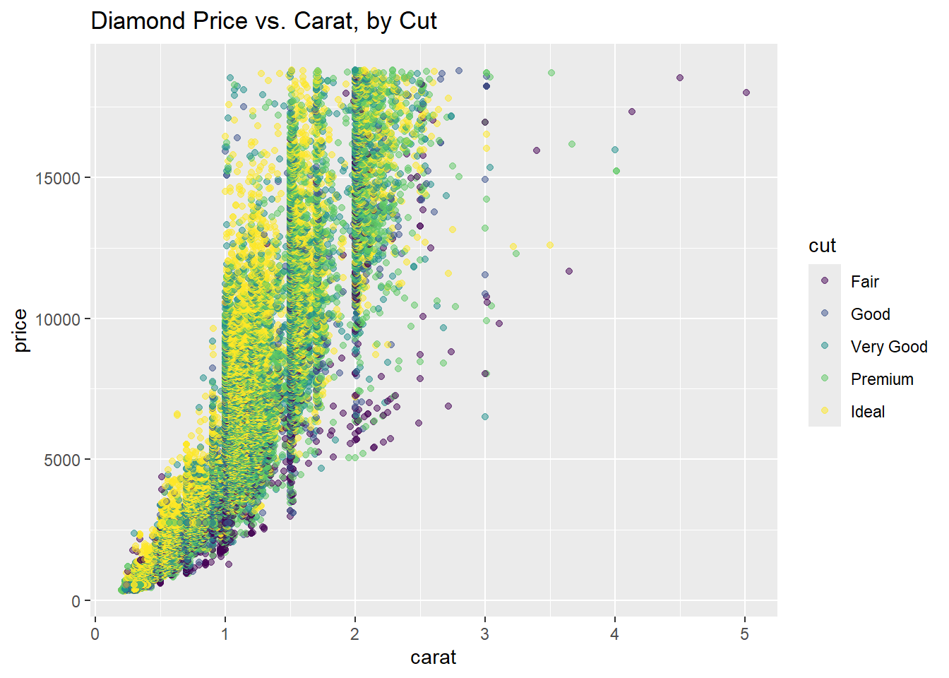
- Do higher-quality cuts tend to cluster at different price or carat ranges?
- How might this influence your interpretation of the relationship between carat and price?
- Fit a multiple regression model for
priceusing bothcaratandcutas Explanatory Variables.
mod2 <- lm(price ~ carat + cut, data = diamonds)
summary(mod2)
Call:
lm(formula = price ~ carat + cut, data = diamonds)

Residuals:
     Min       1Q   Median       3Q      Max
-17540.7   -791.6    -37.6    522.1  12721.4

Coefficients:
            Estimate Std. Error  t value Pr(>|t|)
(Intercept) -2701.38      15.43 -175.061  < 2e-16 ***
carat        7871.08      13.98  563.040  < 2e-16 ***
cut.L        1239.80      26.10   47.502  < 2e-16 ***
cut.Q        -528.60      23.13  -22.851  < 2e-16 ***
cut.C         367.91      20.21   18.201  < 2e-16 ***
cut^4          74.59      16.24    4.593 4.37e-06 ***
---
Signif. codes:  0 '***' 0.001 '**' 0.01 '*' 0.05 '.' 0.1 ' ' 1

Residual standard error: 1511 on 53934 degrees of freedom
Multiple R-squared:  0.8565,    Adjusted R-squared:  0.8565
F-statistic: 6.437e+04 on 5 and 53934 DF, p-value: < 2.2e-16- Write out the multiple regression equation with intercept, coefficients, and variable names.
- Interpret the coefficient for
cutwhile controlling forcarat.
How much total variation in diamond price is explained by this model (i.e., (R^2))?
This model assumes that the effect of carat on price is the same across all cuts.
- How can we check whether this assumption is valid?
Create a multiple regression model for
priceusing bothcaratandcut, including an interaction between them.
mod3 <- lm(price ~ carat * cut, data = diamonds)
summary(mod3)
Call:
lm(formula = price ~ carat * cut, data = diamonds)

Residuals:
     Min       1Q   Median       3Q      Max
-14878.3   -793.0    -23.0    546.3  12706.2

Coefficients:
            Estimate Std. Error  t value Pr(>|t|)
(Intercept) -2271.95      20.94 -108.513  < 2e-16 ***
carat        7468.05      19.49  383.200  < 2e-16 ***
cut.L        -278.21      57.17   -4.866 1.14e-06 ***
cut.Q         363.22      50.51    7.191 6.50e-13 ***
cut.C        -172.96      42.81   -4.041 5.34e-05 ***
cut^4          67.55      33.40    2.022   0.0431 *
carat:cut.L  1538.10      50.96   30.183  < 2e-16 ***
carat:cut.Q  -781.89      45.89  -17.037  < 2e-16 ***
carat:cut.C   509.65      41.36   12.321  < 2e-16 ***
carat:cut^4    69.70      34.38    2.027   0.0426 *
---
Signif. codes:  0 '***' 0.001 '**' 0.01 '*' 0.05 '.' 0.1 ' ' 1

Residual standard error: 1498 on 53930 degrees of freedom
Multiple R-squared:  0.8591,    Adjusted R-squared:  0.859
F-statistic: 3.653e+04 on 9 and 53930 DF,  p-value: < 2.2e-16
Write out the regression equation with intercept, coefficients, and variable names.
\[ \widehat{price} = b_0 + b_1(\text{carat}) + b_2(\text{cut}) + b_3(\text{carat} \times \text{cut}) \]
Among the Ideal cut diamonds, how much does price increase for a one-unit increase in carat?
Among the Fair cut diamonds, how much does price increase for a one-unit increase in carat?
Is the interaction between
caratandcutstatistically significant?- State your null and alternative hypotheses for the interaction term.
- Report the test statistic and p-value.
- State your null and alternative hypotheses for the interaction term.
To what population are you willing to generalize your results?
- Can you draw a cause-and-effect conclusion about carat size and diamond price?
- Why or why not?
- Can you draw a cause-and-effect conclusion about carat size and diamond price?
Check each of the four Validity Conditions for the multiple regression you ran in #8.
- Include all three validity plots for your regression model.
- Justify each of the four conditions: Linearity, Independence, Normality, and Equal Variance.
- Include all three validity plots for your regression model.
Linearity
plot(mod3, which = 1)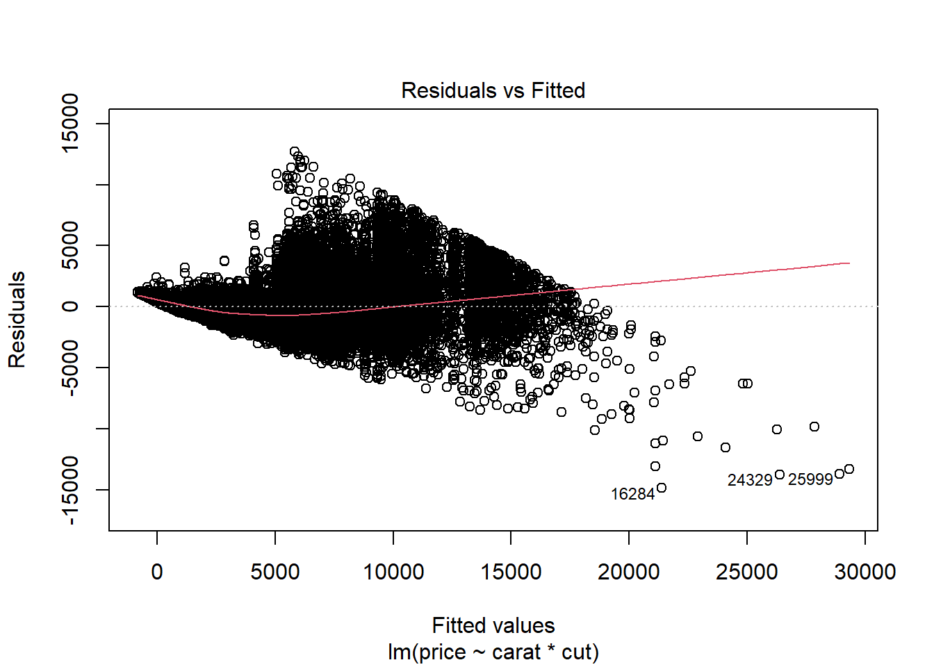
Independence
Must be justified based on data collection (not tested statistically).
Normal Distribution
plot(mod3, which = 2)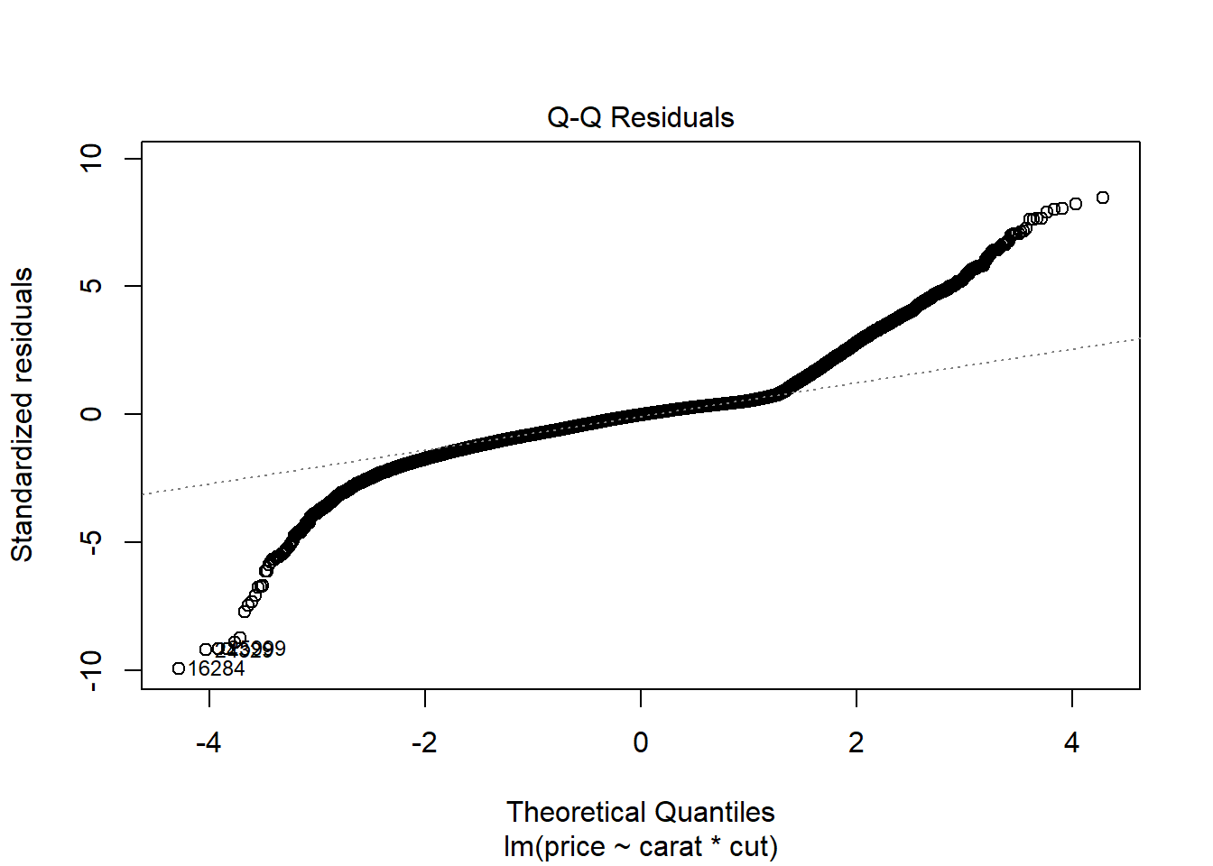
Equal Variance
plot(mod3, which = 1)
Before you leave
Today:
- Any questions for me?