Lesson 10: Binomial Distribution

What We Did: Lessons 6, 7, 8 & 9

Quick Review: Probability Basics (Lesson 6)

Key Concepts from Lesson 6

Sample Spaces and Events:

Sample space \(S\) = set of all possible outcomes
Event = subset of the sample space
Operations: Union (\(A \cup B\)), Intersection (\(A \cap B\)), Complement (\(A^c\))

Kolmogorov Axioms:

\(P(A) \geq 0\)
\(P(S) = 1\)
For mutually exclusive events: \(P(A \cup B) = P(A) + P(B)\)

Key Rules:

Complement Rule: \(P(A^c) = 1 - P(A)\)
Addition Rule: \(P(A \cup B) = P(A) + P(B) - P(A \cap B)\)

Quick Review: Conditional Probability (Lesson 7)

Key Concepts from Lesson 7

Conditional Probability: \[P(A \mid B) = \frac{P(A \cap B)}{P(B)}\]

Multiplication Rule: \[P(A \cap B) = P(A) \cdot P(B \mid A) = P(B) \cdot P(A \mid B)\]

Law of Total Probability: \[P(A) = P(B) \cdot P(A \mid B) + P(B^c) \cdot P(A \mid B^c)\]

Bayes’ Theorem: \[P(B \mid A) = \frac{P(B) \cdot P(A \mid B)}{P(B) \cdot P(A \mid B) + P(B^c) \cdot P(A \mid B^c)}\]

Quick Review: Counting & Independence (Lesson 8)

Key Concepts from Lesson 8

Multiplication Principle: If an experiment has stages with \(n_1, n_2, \ldots, n_k\) outcomes, the total outcomes are \(n_1 \times n_2 \times \cdots \times n_k\).

Counting Formulas:

	With Replacement	Without Replacement
Ordered	\(n^k\)	\(P(n,k) = \frac{n!}{(n-k)!}\)
Unordered	\(\binom{n+k-1}{k}\)	\(\binom{n}{k} = \frac{n!}{k!(n-k)!}\)

Independence:

\(A\) and \(B\) are independent if \(P(A \cap B) = P(A) \cdot P(B)\)
Equivalently: \(P(A \mid B) = P(A)\)
Independent \(\neq\) Mutually Exclusive!

Quick Review: Discrete Random Variables (Lesson 9)

Key Concepts from Lesson 9

Random Variables:

A random variable \(X\) assigns a numerical value to each outcome in a sample space
Discrete RVs take finite or countably infinite values

Probability Mass Function (PMF):

\[p(x) = P(X = x)\]

Properties: \(p(x) \geq 0\) and \(\sum_{\text{all } x} p(x) = 1\)

Cumulative Distribution Function (CDF):

\[F(x) = P(X \leq x) = \sum_{y \leq x} p(y)\]

Key property: CDF is a step function for discrete RVs

What We’re Doing: Lesson 10

Objectives

Verify binomial conditions for counts of successes
Compute binomial PMF/CDF values
Interpret binomial mean and variance

Required Reading

Devore, Section 3.4

Break!

Reese

Cal

Cal and Reese

Finishing Lesson 9: Expected Value and Variance

We didn’t get to cover Expected Value and Variance in Lesson 9, so let’s complete that now using our running example.

Recall: The Coin Flip Example

Example: 3 Fair Coin Flips

A cadet flips a fair coin 3 times.

Let \(X\) = number of heads (out of 3 flips).

PMF (from Lesson 9):

\(x\)	0	1	2	3
\(p(x)\)	\(\frac{1}{8}\)	\(\frac{3}{8}\)	\(\frac{3}{8}\)	\(\frac{1}{8}\)
\(F(x)\)	\(\frac{1}{8}\)	\(\frac{1}{2}\)	\(\frac{7}{8}\)	\(1\)

Expected Value

What if we wanted to know the ‘expected’ number of heads in our coin flip example?

Definition: Expected Value

The expected value (or mean) of a discrete random variable \(X\) is:

\[E(X) = \mu = \sum_{\text{all } x} x \cdot p(x)\]

Interpretation: The expected value is the long-run average — if you repeated the experiment many times, the average value of \(X\) would approach \(E(X)\).

Important Note

The expected value is NOT necessarily a value that \(X\) can actually take!

Expected Value Calculation

\[E(X) = \sum_{x=0}^{3} x \cdot p(x)\]

\[= 0 \cdot \frac{1}{8} + 1 \cdot \frac{3}{8} + 2 \cdot \frac{3}{8} + 3 \cdot \frac{1}{8}\]

\[= 0 + \frac{3}{8} + \frac{6}{8} + \frac{3}{8} = \frac{12}{8} = 1.5\]

Interpretation: On average, you will get 1.5 heads out of 3 flips. Over many repetitions of this experiment, the average number of heads will approach 1.5.

Note: 1.5 is not a possible value of \(X\) (you can’t flip 1.5 heads), but it’s still a meaningful measure of center.

Variance and Standard Deviation

What if we wanted to know how much the number of heads varies between experiments from the expected value?

Definition: Variance

The variance of a discrete random variable \(X\) is:

\[Var(X) = \sigma^2 = E[(X - \mu)^2] = \sum_{\text{all } x} (x - \mu)^2 \cdot p(x)\]

Shortcut formula: \[Var(X) = E(X^2) - [E(X)]^2\]

Definition: Standard Deviation

The standard deviation is:

\[SD(X) = \sigma = \sqrt{Var(X)}\]

Interpretation: Variance and SD measure how spread out the distribution is around the mean.

Variance Calculation: Method 1 (Definition)

\[Var(X) = \sum_{\text{all } x} (x - \mu)^2 \cdot p(x)\]

With \(\mu = 1.5\):

\[ \begin{aligned} Var(X) &= (0 - 1.5)^2 \cdot \frac{1}{8} + (1 - 1.5)^2 \cdot \frac{3}{8} + (2 - 1.5)^2 \cdot \frac{3}{8} + (3 - 1.5)^2 \cdot \frac{1}{8} \\[6pt] &= (2.25) \cdot \frac{1}{8} + (0.25) \cdot \frac{3}{8} + (0.25) \cdot \frac{3}{8} + (2.25) \cdot \frac{1}{8} \\[6pt] &= \frac{2.25}{8} + \frac{0.75}{8} + \frac{0.75}{8} + \frac{2.25}{8} \\[6pt] &= \frac{6}{8} = 0.75 \end{aligned} \]

Variance Calculation: Method 2 (Shortcut Formula)

\[Var(X) = E(X^2) - [E(X)]^2\]

Step 1: Find \(E(X^2)\)

\[ \begin{aligned} E(X^2) &= \sum_{x=0}^{3} x^2 \cdot p(x) \\[6pt] &= 0^2 \cdot \frac{1}{8} + 1^2 \cdot \frac{3}{8} + 2^2 \cdot \frac{3}{8} + 3^2 \cdot \frac{1}{8} \\[6pt] &= 0 + \frac{3}{8} + \frac{12}{8} + \frac{9}{8} = \frac{24}{8} = 3 \end{aligned} \]

Step 2: Apply the shortcut formula

\[Var(X) = E(X^2) - [E(X)]^2 = 3 - (1.5)^2 = 3 - 2.25 = 0.75\]

Standard Deviation

\[SD(X) = \sqrt{Var(X)} = \sqrt{0.75} \approx 0.866\]

Interpretation: The number of heads typically varies by about 0.87 from the average of 1.5.

Summary: Coin Flip Example Complete

Complete Analysis: 3 Fair Coin Flips

PMF and CDF:

\(x\)	0	1	2	3
\(p(x)\)	\(\frac{1}{8}\)	\(\frac{3}{8}\)	\(\frac{3}{8}\)	\(\frac{1}{8}\)
\(F(x)\)	\(\frac{1}{8}\)	\(\frac{1}{2}\)	\(\frac{7}{8}\)	\(1\)

Summary Statistics:

\(E(X) = 1.5\) heads
\(Var(X) = 0.75\)
\(SD(X) \approx 0.866\) heads

The Takeaway for Today

Key Concepts: Binomial Distribution

The Four Binomial Conditions (BINS):

Binary outcomes: Each trial has exactly two outcomes (success/failure)
Independent trials: The outcome of one trial doesn’t affect others
Number of trials is fixed: You know \(n\) in advance
Same probability: The probability of success \(p\) is constant for each trial

Key Formulas:

PMF: \(P(X = x) = \binom{n}{x} p^x (1-p)^{n-x}\)
Mean: \(E(X) = np\)
Variance: \(Var(X) = np(1-p)\)

R Functions:

dbinom(x, size = n, prob = p) — PMF: \(P(X = x)\)
pbinom(x, size = n, prob = p) — CDF: \(P(X \leq x)\)

Lets Re-Think Our Coin Flipping Experiment

Board Work: From Coin Flips to the Binomial Formula

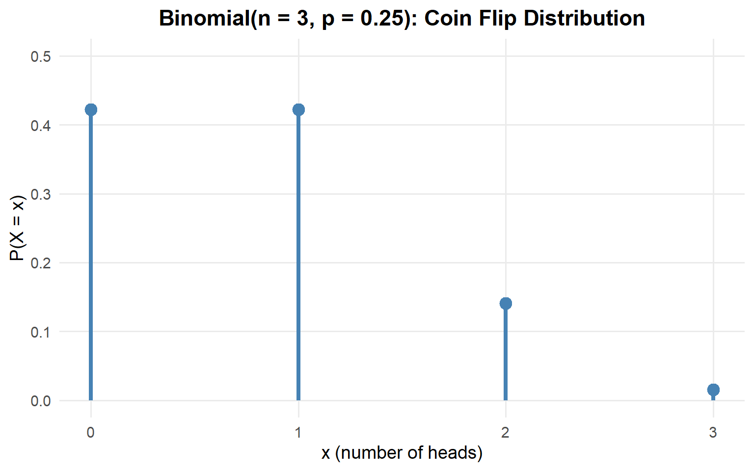
Remember our coin flipping example from Lesson 9? We had \(n = 3\) flips of a fair coin (\(p = 0.5\)).

What if \(p = 0.25\) instead of \(0.5\)?

Outcome	Probability	=
HHH	\((.25)(.25)(.25)\)	\(\frac{1}{64}\)
HHT	\((.25)(.25)(.75)\)	\(\frac{3}{64}\)
HTH	\((.25)(.75)(.25)\)	\(\frac{3}{64}\)
HTT	\((.25)(.75)(.75)\)	\(\frac{9}{64}\)
THH	\((.75)(.25)(.25)\)	\(\frac{3}{64}\)
THT	\((.75)(.25)(.75)\)	\(\frac{9}{64}\)
TTH	\((.75)(.75)(.25)\)	\(\frac{9}{64}\)
TTT	\((.75)(.75)(.75)\)	\(\frac{27}{64}\)

Find \(P(X = x)\) by listing all outcomes

\(x\)	0	1	2	3
\(p(x)\)	\(\frac{27}{64}\)	\(\frac{27}{64}\)	\(\frac{9}{64}\)	\(\frac{1}{64}\)

That’s terrible… let’s make this into a formula…

How many ways can we select \(x\) heads from \(n\) coin flips?

\[\binom{n}{x}\]

What’s the probability of each of those arrangements happening?

\[p^x (1-p)^{n-x}\]

Putting it together:

\[P(X = x) = \binom{n}{x} p^x (1-p)^{n-x}\]

This is known as a Binomial Experiment

The Setup

Imagine an experiment where:

You perform the same action \(n\) times (like n coin flips)
Each trial has only two possible outcomes: success or failure (or heads or tails)
The probability of success \(p\) stays the same for each trial (like .25)
The trials are independent of each other (like coin flips are)

This is called a binomial experiment.

The Four Binomial Conditions (BINS)

BINS: Four Conditions for a Binomial Experiment

Binary outcomes: Each trial results in one of exactly two outcomes
- Success (what we’re counting) or Failure
Independent trials: The outcome of one trial doesn’t affect other trials
- Knowing one result doesn’t change probabilities for other trials
Number of trials is fixed: We know \(n\) before the experiment starts
- We’re not stopping when something happens
Same probability: \(P(\text{success}) = p\) is constant across all trials
- The probability doesn’t change from trial to trial

If all four conditions are met, then \(X\) = number of successes follows a binomial distribution.

Examples: Check BINS

Scenario 1: A cadet attempts 10 free throws. Each shot has a 70% chance of going in, and the results of each shot are independent. Let \(X\) = number of made shots.

Check BINS

Binary? ✓ Each shot is either made (success) or missed (failure)
Independent? ✓ Each shot’s outcome doesn’t affect the others
Number fixed? ✓ We know there will be exactly 10 shots
Same probability? ✓ Each shot has 70% success probability

\(X \sim \text{Binomial}(n=10, p=0.7)\)

Scenario 2: Draw 5 cards from a deck without replacement. Let \(X\) = number of hearts.

Check BINS

Binary? ✓ Each card is either a heart (success) or not (failure)
Independent? ✓ Each draw is independent… wait, is it?
Number fixed? ✓ We know there will be exactly 5 draws
Same probability? ✗ The probability changes with each draw
- First draw: \(P(\text{heart}) = 13/52\)
- If first was a heart: \(P(\text{heart on second}) = 12/51\)
- If first was not a heart: \(P(\text{heart on second}) = 13/51\)

Not binomial.

Scenario 3: Roll a die until you get a 6. Let \(X\) = number of rolls.

Check BINS

Binary? ✓ Each roll is either a 6 (success) or not (failure)
Independent? ✓ Each roll is independent
Number fixed? ✗ We don’t know how many rolls it will take
Same probability? ✓ Each roll has \(p = 1/6\)

Not binomial.

The Binomial Distribution

The Binomial PMF

If \(X \sim \text{Binomial}(n, p)\), then the probability of exactly \(x\) successes is:

\[P(X = x) = \binom{n}{x} p^x (1-p)^{n-x}, \quad x = 0, 1, 2, \ldots, n\]

where:

\(\binom{n}{x}\) = number of ways to arrange \(x\) successes among \(n\) trials
\(p^x\) = probability of \(x\) successes (each with probability \(p\))
\((1-p)^{n-x}\) = probability of \(n-x\) failures (each with probability \(1-p\))

Using the PMF: Our Coin Flip Example

Let’s verify our earlier work using the formula. For \(n = 3\) flips with \(p = 0.25\):

\[P(X = 0) = \binom{3}{0} (0.25)^0 (0.75)^3 = 1 \cdot 1 \cdot \frac{27}{64} = \frac{27}{64}\]

\[P(X = 1) = \binom{3}{1} (0.25)^1 (0.75)^2 = 3 \cdot \frac{1}{4} \cdot \frac{9}{16} = \frac{27}{64}\]

\[P(X = 2) = \binom{3}{2} (0.25)^2 (0.75)^1 = 3 \cdot \frac{1}{16} \cdot \frac{3}{4} = \frac{9}{64}\]

\[P(X = 3) = \binom{3}{3} (0.25)^3 (0.75)^0 = 1 \cdot \frac{1}{64} \cdot 1 = \frac{1}{64}\]

These match what we found by enumeration!

What about \(P(X \leq 2)\)?

\[P(X \leq 2) = \sum_{x=0}^{2} \binom{3}{x} (0.25)^x (0.75)^{3-x} = P(X=0) + P(X=1) + P(X=2)\]

\[= \frac{27}{64} + \frac{27}{64} + \frac{9}{64} = \frac{63}{64}\]

Visualizing the Binomial Distribution

Binomial Calculations in R

The dbinom() Function: PMF

The dbinom() function computes \(P(X = x)\) — the probability of exactly \(x\) successes.

# P(X = 2) when n = 4 and p = 0.7
dbinom(2, size = 4, prob = 0.7)

[1] 0.2646

Compare to our hand calculation: \(\binom{4}{2}(0.7)^2(0.3)^2 = 6 \times 0.49 \times 0.09 = 0.2646\) ✓

The pbinom() Function: CDF

The pbinom() function computes \(P(X \leq x)\) — the probability of \(x\) or fewer successes.

# P(X ≤ 2) when n = 4 and p = 0.7
pbinom(2, size = 4, prob = 0.7)

[1] 0.3483

This equals \(P(X=0) + P(X=1) + P(X=2)\).

Common Probability Calculations

Example: \(X \sim \text{Binomial}(n=4, p=0.7)\)

P(X = 3): Probability of exactly 3 successes

\[P(X = 3) = \binom{4}{3} (0.7)^3 (0.3)^1\]

dbinom(3, size = 4, prob = 0.7)

[1] 0.4116

P(X ≤ 2): Probability of 2 or fewer successes

\[P(X \leq 2) = \sum_{x=0}^{2} \binom{4}{x} (0.7)^x (0.3)^{4-x}\]

pbinom(2, size = 4, prob = 0.7)

[1] 0.3483

P(X < 2): Probability of fewer than 2 successes

\[P(X < 2) = P(X \leq 1) = \sum_{x=0}^{1} \binom{4}{x} (0.7)^x (0.3)^{4-x}\]

pbinom(1, size = 4, prob = 0.7)

[1] 0.0837

P(X > 2): Probability of more than 2 successes

\[P(X > 2) = 1 - P(X \leq 2) = 1 - \sum_{x=0}^{2} \binom{4}{x} (0.7)^x (0.3)^{4-x}\]

1 - pbinom(2, size = 4, prob = 0.7)

[1] 0.6517

P(X ≥ 2): Probability of 2 or more successes

\[P(X \geq 2) = 1 - P(X \leq 1) = 1 - \sum_{x=0}^{1} \binom{4}{x} (0.7)^x (0.3)^{4-x}\]

1 - pbinom(1, size = 4, prob = 0.7)

[1] 0.9163

Mean and Variance of the Binomial

Formulas

Mean and Variance of Binomial Distribution

If \(X \sim \text{Binomial}(n, p)\), then:

\[E(X) = \mu = np\]

\[Var(X) = \sigma^2 = np(1-p)\]

\[SD(X) = \sigma = \sqrt{np(1-p)}\]

Why \(E(X) = np\)? Intuition: If you flip a fair coin 100 times, you expect about 50 heads. If each trial has probability \(p\) of success, and you do \(n\) trials, you expect about \(np\) successes.

Example: Free Throw Stats

For our free throw shooter with \(n = 4\) shots and \(p = 0.7\):

\[E(X) = np = 4 \times 0.7 = 2.8\]

\[Var(X) = np(1-p) = 4 \times 0.7 \times 0.3 = 0.84\]

\[SD(X) = \sqrt{0.84} \approx 0.917\]

Interpretation:

On average, the player makes 2.8 shots out of 4
The typical deviation from this average is about 0.92 shots

Connection to Our Coin Flip Example

Remember our 3 coin flips with \(p = 0.25\)?

That’s binomial with \(n=3\) and \(p=0.25\).

\[E(X) = np = 3 \times 0.25 = 0.75\]

\[Var(X) = np(1-p) = 3 \times 0.25 \times 0.75 = 0.5625\]

\[SD(X) = \sqrt{0.5625} = 0.75\]

The binomial formulas make these calculations quick!

Board Problems

Class Problem: Land Navigation

A cadet completes 16 land navigation points. Each point has a 50% chance of being found successfully, independent of the others. Let \(X\) = number of points found.

Verify this is a binomial setting (check BINS)

Binary? ✓ Each point is either found or not
Independent? ✓ Finding one point doesn’t affect finding another
Number fixed? ✓ There are exactly 16 points
Same probability? ✓ Each has 50% chance of being found

\(X \sim \text{Binomial}(n=16, p=0.5)\)

What are E(X) and SD(X)?

\[E(X) = np = 16 \times 0.5 = 8\]

\[SD(X) = \sqrt{np(1-p)} = \sqrt{16 \times 0.5 \times 0.5} = \sqrt{4} = 2\]

On average, 8 points will be found, with a typical deviation of 2 points.

What is the probability X is within 1 SD of the mean?

Within 1 SD means: \(\mu - \sigma \leq X \leq \mu + \sigma\), so \(8 - 2 \leq X \leq 8 + 2\)

\[P(6 \leq X \leq 10) = P(X \leq 10) - P(X \leq 5)\]

pbinom(10, size = 16, prob = 0.5) - pbinom(5, size = 16, prob = 0.5)

[1] 0.7898865

What is the probability X is within 2 SDs of the mean?

Within 2 SDs means: \(\mu - 2\sigma \leq X \leq \mu + 2\sigma\), so \(8 - 4 \leq X \leq 8 + 4\)

\[P(4 \leq X \leq 12) = P(X \leq 12) - P(X \leq 3)\]

pbinom(12, size = 16, prob = 0.5) - pbinom(3, size = 16, prob = 0.5)

[1] 0.9787292

What is the probability X is more than 2 SDs from the mean?

More than 2 SDs from the mean means \(X < 4\) or \(X > 12\)

\[P(X < 4 \text{ or } X > 12) = 1 - P(4 \leq X \leq 12)\]

1 - (pbinom(12, size = 16, prob = 0.5) - pbinom(3, size = 16, prob = 0.5))

[1] 0.02127075

Problem 2: Rifle Qualification

At a rifle qualification range, historical data shows that 85% of cadets qualify as “Expert” on their first attempt.

A platoon of 12 cadets attempts the qualification. Let \(X\) = number who qualify Expert.

Verify this is a binomial setting (check BINS)

Binary? ✓ Each cadet either qualifies Expert or doesn’t
Independent? ✓ One cadet’s performance doesn’t affect another’s
Number fixed? ✓ There are exactly 12 cadets
Same probability? ✓ Each has 85% chance of qualifying Expert

\(X \sim \text{Binomial}(n=12, p=0.85)\)

What are E(X) and SD(X)?

\[E(X) = np = 12 \times 0.85 = 10.2\]

\[SD(X) = \sqrt{np(1-p)} = \sqrt{12 \times 0.85 \times 0.15} = \sqrt{1.53} \approx 1.24\]

On average, 10.2 cadets will qualify Expert, with a typical deviation of about 1.24.

What is the probability exactly 10 qualify Expert?

\[P(X = 10) = \binom{12}{10}(0.85)^{10}(0.15)^{2}\]

dbinom(10, size = 12, prob = 0.85)

[1] 0.2923585

What is the probability all 12 qualify Expert?

\[P(X = 12) = \binom{12}{12}(0.85)^{12}(0.15)^{0} = (0.85)^{12}\]

dbinom(12, size = 12, prob = 0.85)

[1] 0.1422418

What is the probability at least 10 qualify Expert?

\[P(X \geq 10) = P(X = 10) + P(X = 11) + P(X = 12) = 1 - P(X \leq 9)\]

1 - pbinom(9, size = 12, prob = 0.85)

[1] 0.7358181

Problem 3: Equipment Readiness

A motor pool has 20 vehicles. Each vehicle has a 90% probability of being fully mission capable (FMC) on any given day, independent of others.

What is the probability exactly 18 vehicles are FMC?

\(X \sim \text{Binomial}(n=20, p=0.90)\)

dbinom(18, size = 20, prob = 0.90)

[1] 0.2851798

What is the probability at least 18 are FMC?

\[P(X \geq 18) = 1 - P(X \leq 17)\]

1 - pbinom(17, size = 20, prob = 0.90)

[1] 0.6769268

The commander needs at least 16 vehicles for an operation. What is the probability the motor pool can support this?

\[P(X \geq 16) = 1 - P(X \leq 15)\]

1 - pbinom(15, size = 20, prob = 0.90)

[1] 0.9568255

Problem 4: PT Test Pass Rates

In a company, 75% of soldiers pass the ACFT on their first attempt. A random sample of 8 soldiers is selected.

What are the mean and standard deviation of the number who pass?

\(X \sim \text{Binomial}(n=8, p=0.75)\)

\[E(X) = 8 \times 0.75 = 6\]

\[SD(X) = \sqrt{8 \times 0.75 \times 0.25} = \sqrt{1.5} \approx 1.22\]

What is the probability fewer than half pass?

\[P(X < 4) = P(X \leq 3)\]

pbinom(3, size = 8, prob = 0.75)

[1] 0.02729797

What is the probability at least 6 pass?

\[P(X \geq 6) = 1 - P(X \leq 5)\]

1 - pbinom(5, size = 8, prob = 0.75)

[1] 0.6785431

Problem 5: Drone Reliability

A reconnaissance drone has a 95% success rate for each mission. If the unit conducts 15 missions:

What is the expected number of successful missions?

\(X \sim \text{Binomial}(n=15, p=0.95)\)

\[E(X) = np = 15 \times 0.95 = 14.25\]

What is the probability all 15 missions are successful?

dbinom(15, size = 15, prob = 0.95)

[1] 0.4632912

What is the probability at most 2 missions fail?

At most 2 failures means at least 13 successes: \(P(X \geq 13)\)

1 - pbinom(12, size = 15, prob = 0.95)

[1] 0.9637998

Before You Leave

Today

Finished Lesson 9: Expected Value and Variance for discrete RVs
The Binomial distribution models counts of successes in fixed trials
BINS conditions: Binary, Independent, Number fixed, Same probability
Binomial PMF: \(P(X = x) = \binom{n}{x}p^x(1-p)^{n-x}\)
Mean: \(E(X) = np\), Variance: \(Var(X) = np(1-p)\)
R functions: dbinom() for PMF, pbinom() for CDF

Any questions?

Next Lesson

Lesson 11: Poisson Distribution

The Poisson distribution for rare events
Poisson as approximation to Binomial
Mean and variance of Poisson

Upcoming Graded Events

WebAssign 3.4 - Due before Lesson 11
WPR I - Lesson 16