
Lesson 24: Paired t-Test
WarningCAC
We are getting into Army Vantage today. Bring your CAC / military ID into class.
What We Did: Lessons 17–23
NoteLesson 17: Central Limit Theorem
The Central Limit Theorem (CLT): If \(X_1, X_2, \ldots, X_n\) are iid with mean \(\mu\) and standard deviation \(\sigma\), then for large \(n\):
\[\bar{X} \sim N\left(\mu, \frac{\sigma^2}{n}\right)\]
Standard Error of the Mean: \(\sigma_{\bar{X}} = \frac{\sigma}{\sqrt{n}}\)
Rule of thumb: \(n \geq 30\) unless the population is already normal.
NoteLesson 18: Confidence Intervals I
Confidence Interval for a Mean:
| Formula | When to Use | |
|---|---|---|
| Large sample (\(n \geq 30\)) | \(\bar{X} \pm z_{\alpha/2} \cdot \dfrac{\sigma}{\sqrt{n}}\) | Random sample, independence, \(s \approx \sigma\) |
| Small sample (\(n < 30\)) | \(\bar{X} \pm t_{\alpha/2, n-1} \cdot \dfrac{s}{\sqrt{n}}\) | Random sample, independence, population ~ Normal |
Key ideas: Higher confidence → wider interval. Larger \(n\) → narrower interval.
NoteLesson 19: Confidence Intervals II
Confidence Interval for a Proportion:
\[\hat{p} \pm z_{\alpha/2} \cdot \sqrt{\frac{\hat{p}(1-\hat{p})}{n}}\]
Conditions: \(n\hat{p} \geq 10\) and \(n(1-\hat{p}) \geq 10\)
Interpretation: “We are C% confident that [interval] captures the true [parameter in context].” The confidence level describes the method’s long-run success rate, not the probability any single interval is correct.
NoteLesson 20: Intro to Hypothesis Testing
Every hypothesis test follows four steps:
- State hypotheses: \(H_0\) (null — status quo) vs. \(H_a\) (alternative — what we want to show)
- Compute a test statistic: How far is our sample result from what \(H_0\) predicts?
- Find the \(p\)-value: If \(H_0\) were true, how likely is a result this extreme or more?
- Make a decision: If \(p \leq \alpha\), reject \(H_0\). If \(p > \alpha\), fail to reject \(H_0\).
NoteLesson 21: One Sample t-Test & One-Proportion z-Test
One-sample \(t\)-test for a mean (\(\sigma\) unknown):
\[t = \frac{\bar{x} - \mu_0}{s / \sqrt{n}}, \qquad df = n - 1\]
One-proportion \(z\)-test:
\[z = \frac{\hat{p} - p_0}{\sqrt{\dfrac{p_0(1 - p_0)}{n}}}\]
Conditions for proportions: \(np_0 \geq 10\) and \(n(1-p_0) \geq 10\) (use \(p_0\), not \(\hat{p}\)!)
NoteLesson 22: Two-Sample z-Test (Large Samples)
Two-sample \(z\)-test for means (\(n_1 \geq 30\) and \(n_2 \geq 30\)):
\[z = \frac{(\bar{x}_1 - \bar{x}_2) - \Delta_0}{\sqrt{\dfrac{s_1^2}{n_1} + \dfrac{s_2^2}{n_2}}}\]
Conditions: Large samples (\(n_1, n_2 \geq 30\)), random samples from two separate groups.
CI for \(\mu_1 - \mu_2\): \((\bar{x}_1 - \bar{x}_2) \pm z_{\alpha/2} \cdot SE\)
NoteLesson 23: Two-Sample t-Test (Small Samples)
Two-sample \(t\)-test (small samples): Same formula as the \(z\)-test, but use \(t\)-distribution:
\[t = \frac{(\bar{x}_1 - \bar{x}_2) - \Delta_0}{\sqrt{\dfrac{s_1^2}{n_1} + \dfrac{s_2^2}{n_2}}}, \qquad df = \frac{\left(\dfrac{s_1^2}{n_1} + \dfrac{s_2^2}{n_2}\right)^2}{\dfrac{\left(s_1^2/n_1\right)^2}{n_1 - 1} + \dfrac{\left(s_2^2/n_2\right)^2}{n_2 - 1}}\]
Conditions: Random samples from two separate groups, both populations approximately normal.
What We’re Doing: Lesson 24
Objectives
- Identify paired versus not-paired designs
- Test a mean difference using the paired \(t\)-test
- Construct and interpret a confidence interval for a mean difference
Required Reading
Devore, Section 9.3
WPR II Information
ImportantWPR II — Lesson 27
- Review: 175 points — look at your WPR I to see what we told you before the WPR
- Covers: Concepts from Lessons 17–26
- Time: 55 minutes
- Authorized: Course Statistics Reference Card (SRC) and the issued calculator
- Technology — R-Lite (
pt,qt,pnorm,qnormonly), no internet, no electronic devices - Round all numbers to three significant digits
Break!

Reese


Cal

The Takeaway for Today
ImportantToday’s Key Ideas
Paired data arise when the same subjects are measured twice (or matched one-to-one). The key move: compute differences, then it’s a one-sample \(t\)-test.
\[t = \frac{\bar{d} - \Delta_0}{s_d / \sqrt{n}}, \qquad df = n - 1\]
CI for \(\mu_d\):
\[\bar{d} \pm t_{\alpha/2, \, n-1} \cdot \frac{s_d}{\sqrt{n}}\]
Why pair? Pairing removes between-subject variability, giving the test more power to detect a real effect.
Review: Two-Sample t-Test
Let’s make sure we’re solid on what we learned last class before we introduce today’s new idea.
Review Problem: Body Armor Weight
Two companies test different body armor configurations. The S4 wants to know if there’s a difference in average load weight. Different Soldiers in each group — no connection between individuals.
| Config A | Config B | |
|---|---|---|
| \(n\) | 10 | 12 |
| \(\bar{x}\) (lbs) | 34.2 | 31.8 |
| \(s\) | 3.5 | 4.1 |
Step 1: State the Hypotheses
\[H_0: \mu_A - \mu_B = 0 \qquad \text{vs.} \qquad H_a: \mu_A - \mu_B \neq 0\]
Step 2: Compute the Test Statistic
\[t = \frac{(\bar{x}_1 - \bar{x}_2) - \Delta_0}{\sqrt{\dfrac{s_1^2}{n_1} + \dfrac{s_2^2}{n_2}}} = \frac{(34.2 - 31.8) - 0}{\sqrt{\dfrac{3.5^2}{10} + \dfrac{4.1^2}{12}}} = \frac{2.4}{\sqrt{1.225 + 1.401}} = \frac{2.4}{\sqrt{2.626}} = \frac{2.4}{1.621} = 1.48\]
n1 <- 10; n2 <- 12
xbar1 <- 34.2; xbar2 <- 31.8
s1 <- 3.5; s2 <- 4.1

se <- sqrt(s1^2 / n1 + s2^2 / n2)
t_stat <- (xbar1 - xbar2) / se
t_stat
[1] 1.481077Degrees of freedom: Now we need \(df\) to find the \(p\)-value. There are a few ways to get it:
NoteThree Ways to Get Degrees of Freedom
| Method | Formula | \(df\) for this problem |
|---|---|---|
| Equal variances assumed | \(df = n_1 + n_2 - 2\) | \(10 + 12 - 2 = 20\) |
| Conservative (quick) | \(df = \min(n_1 - 1, \, n_2 - 1)\) | \(\min(9, 11) = 9\) |
| Welch (exact) | \(df = \dfrac{\left(\dfrac{s_1^2}{n_1} + \dfrac{s_2^2}{n_2}\right)^2}{\dfrac{\left(s_1^2/n_1\right)^2}{n_1 - 1} + \dfrac{\left(s_2^2/n_2\right)^2}{n_2 - 1}}\) | \(\lfloor 19.98 \rfloor = 19\) |
- If you can assume equal variances (\(s_1 \approx s_2\)), use \(n_1 + n_2 - 2\). Simple.
- If you want a quick, safe answer by hand, use \(\min(n_1 - 1, n_2 - 1)\). This is conservative — it gives you fewer degrees of freedom, which makes it harder to reject \(H_0\).
- The Welch formula is the most accurate when variances differ.
We’ll use the conservative approach: \(df = \min(10 - 1, \, 12 - 1) = \min(9, 11) = 9\).
df <- min(n1 - 1, n2 - 1)
df
[1] 9Step 3: Find the \(p\)-Value
Two-tailed with \(df = 9\):
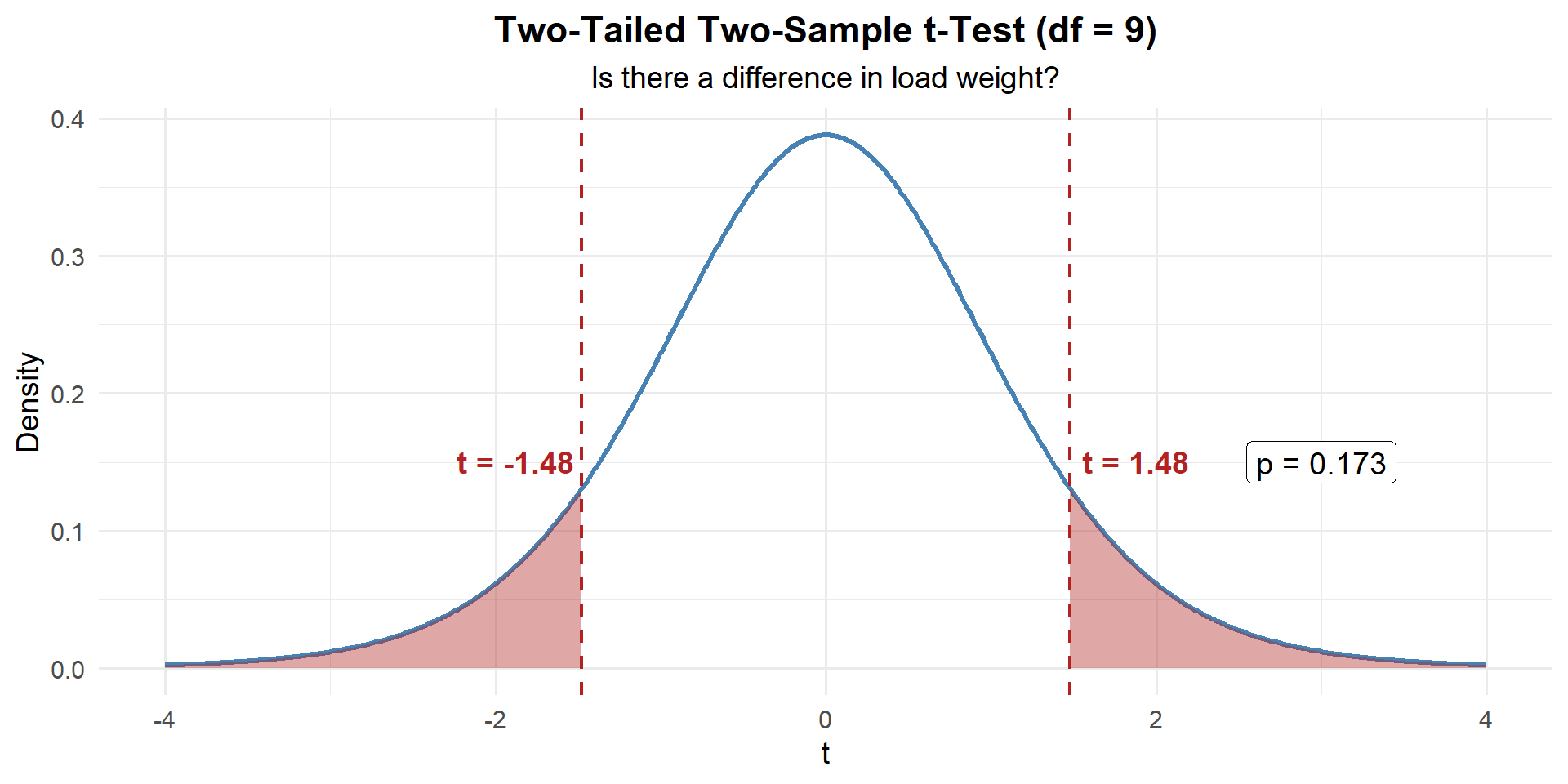
p_value <- 2 * (1 - pt(abs(t_stat), df = df))
p_value
[1] 0.1727239Step 4: Decide and Conclude
\(p = 0.1727 > 0.05\), so we fail to reject \(H_0\). There is not sufficient evidence of a difference in average load weight between the two configurations.
That’s the two-sample \(t\)-test we already know. Different people in each group, no natural pairing.
But What If We Had This Scenario Instead?
What if instead of two separate groups of Soldiers wearing different armor, we had the same 10 Soldiers each test both configurations?
Or think about these situations:
- Same Soldiers’ AFT scores before and after a training program
- Same cadets’ performance on two different tasks
- Same rifles tested with old vs. new cleaning method
- Same patients’ blood pressure before and after medication
In each case, the two measurements come from the same individuals. A Soldier who scores high before training will probably score high after, too. The two measurements are not from separate groups — they’re paired.
ImportantHow to Tell: Paired or Not-Paired?
Ask yourself: Is there a natural one-to-one pairing between the observations?
- Paired: Same person measured twice, left vs. right, before vs. after, matched subjects
- Not-paired: Two separate groups with no connection between individual observations
| Scenario | Design |
|---|---|
| 50 Soldiers’ AFT scores before and after a PT program | Paired |
| 30 cadets from Co A vs. 35 cadets from Co B on a math exam | Not-paired |
| 20 rifles tested with old method, then same 20 with new method | Paired |
| Reaction times of 25 caffeine users vs. 25 non-users | Not-paired |
| Each of 25 cadets rates difficulty of two courses | Paired |
So how do we handle paired data? We can’t use the two-sample \(t\)-test — it assumes the groups are not paired.
The Key Insight: Just Compute Differences
Here’s the beautiful thing. Watch what happens when we compute the differences:
| Soldier | Before | After | \(d_i = \text{After} - \text{Before}\) |
|---|---|---|---|
| 1 | 445 | 460 | 15 |
| 2 | 478 | 491 | 13 |
| 3 | 512 | 520 | 8 |
| … | … | … | … |
You started with two columns. Now you have one column of numbers.
And you already know what to do with one column of numbers — that’s a one-sample \(t\)-test from Lesson 21!
The question “Did scores improve?” becomes “Is the mean of these differences greater than zero?”
NoteWait… This Is Just a One-Sample t-Test!
The paired \(t\)-test is not a new test. It’s the exact same one-sample \(t\)-test you already know, applied to the differences.
One-sample \(t\)-test (Lesson 21):
\[t = \frac{\bar{x} - \mu_0}{s / \sqrt{n}}, \qquad df = n - 1\]
Paired \(t\)-test (today):
\[t = \frac{\bar{d} - \Delta_0}{s_d / \sqrt{n}}, \qquad df = n - 1\]
Same formula. Same degrees of freedom. Same pt() for the \(p\)-value. The only thing that changed is that \(\bar{x}\) became \(\bar{d}\) — because your “sample” is now the vector of differences.
Example 1: AFT Scores Before and After a PT Program
A company commander puts 10 Soldiers through a new 6-week PT program:
| Soldier | 1 | 2 | 3 | 4 | 5 | 6 | 7 | 8 | 9 | 10 |
|---|---|---|---|---|---|---|---|---|---|---|
| Before | 345 | 378 | 412 | 290 | 367 | 401 | 323 | 389 | 355 | 338 |
| After | 351 | 383 | 408 | 304 | 371 | 395 | 334 | 395 | 361 | 342 |
Compute the differences:
before <- c(345, 378, 412, 290, 367, 401, 323, 389, 355, 338)
after  <- c(351, 383, 408, 304, 371, 395, 334, 395, 361, 342)
d <- after - before
d
[1] 6 5 -4 14 4 -6 11 6 6 4Now we have a single vector of numbers. From here it’s a one-sample \(t\)-test.
Step 1: State the Hypotheses
Did scores improve? That means \(\mu_d > 0\):
\[H_0: \mu_d = 0 \qquad \text{vs.} \qquad H_a: \mu_d > 0\]
Step 2: Compute the Test Statistic (one-sample \(t\) on the differences)
\[t = \frac{\bar{d} - \Delta_0}{s_d / \sqrt{n}} = \frac{4.6 - 0}{5.985 / \sqrt{10}} = \frac{4.6}{1.893} = 2.430\]
n <- length(d)
d_bar <- mean(d)
s_d <- sd(d)
t_stat <- (d_bar - 0) / (s_d / sqrt(n))
t_stat
[1] 2.430421Step 3: Find the \(p\)-Value
\(df = n - 1 = 9\) — same as any one-sample \(t\)-test:
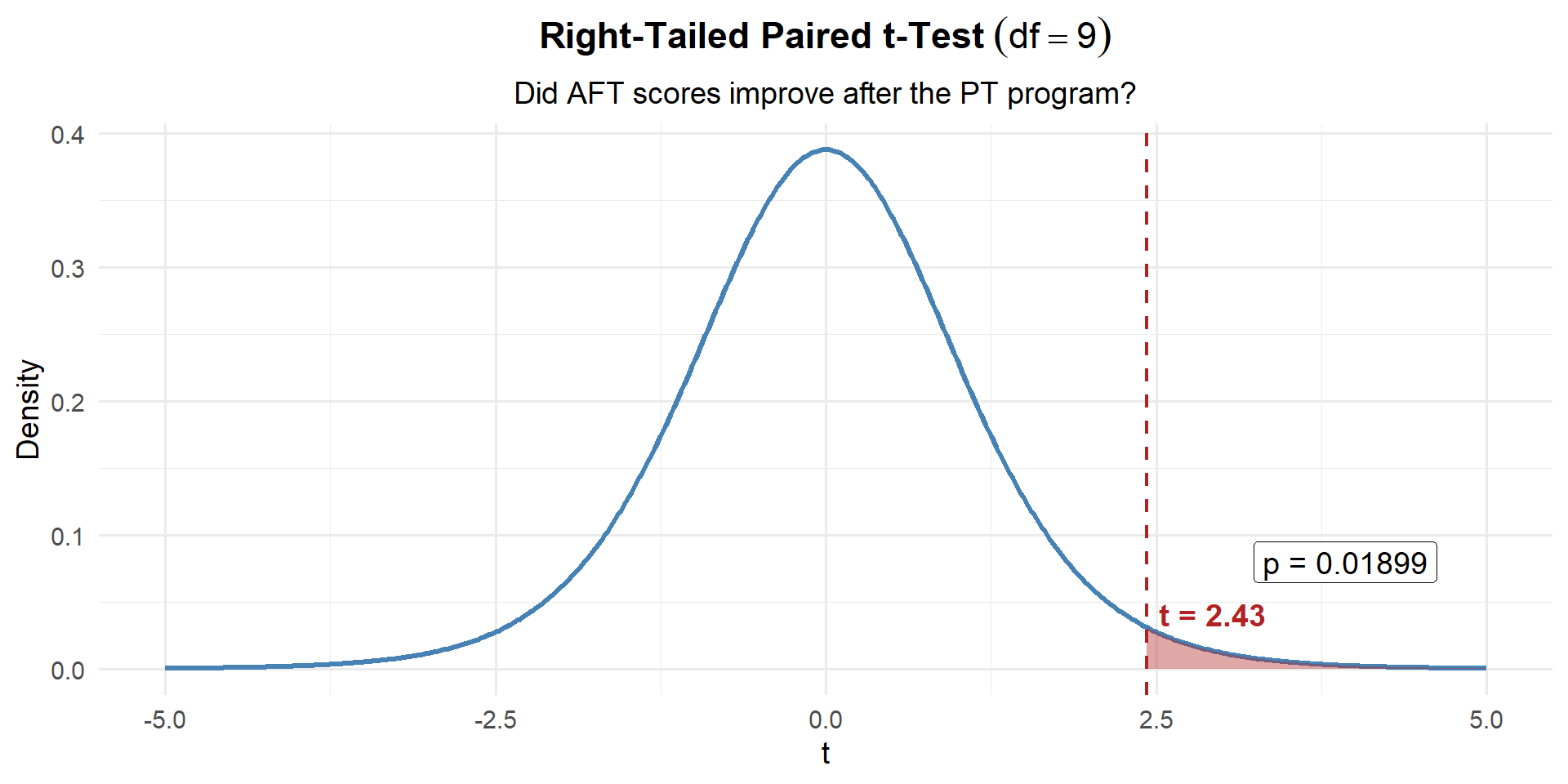
p_value <- 1 - pt(t_stat, df = n - 1)
p_value
[1] 0.01897816Step 4: Decide and Conclude
\(p = 0.01898 \leq 0.05\). We reject \(H_0\). At the 5% significance level, there is strong evidence that the PT program improved AFT scores. The average improvement was 4.6 points.
Confidence Interval for the Mean Difference
Just like any one-sample \(t\) CI:
\[\bar{d} \pm t_{\alpha/2, \, n-1} \cdot \frac{s_d}{\sqrt{n}}\]
t_crit <- qt(0.975, df = n - 1)
me <- t_crit * s_d / sqrt(n)
c(d_bar - me, d_bar + me)
[1] 0.3184696 8.8815304We are 95% confident that the true average AFT improvement is between 0.3 and 8.9 points.
Since the entire interval is above zero, this is consistent with rejecting \(H_0\).
Why Pairing Matters
What would happen if we ignored the pairing and ran a two-sample \(t\)-test on this data? We’d treat 445 and 460 as if they came from unrelated people. All that natural person-to-person variability — some Soldiers are naturally at 500, some at 400 — would inflate our standard error, making it harder to detect a real effect.
By pairing, each Soldier is their own control. The only variability left is in the differences — did each Soldier improve? That’s a much cleaner signal.
WarningBottom Line
If the data are paired, use a paired test. Ignoring the pairing wastes information and can cause you to miss a real effect.
Example 2: Rifle Qualification with New Sights
A platoon sergeant wants to know if switching to a new optic changes marksmanship scores. 12 Soldiers shoot a qualification with their current sights, then again with the new optic:
| Soldier | 1 | 2 | 3 | 4 | 5 | 6 | 7 | 8 | 9 | 10 | 11 | 12 |
|---|---|---|---|---|---|---|---|---|---|---|---|---|
| Current | 31 | 28 | 35 | 26 | 33 | 29 | 37 | 30 | 27 | 32 | 34 | 25 |
| New | 33 | 27 | 36 | 28 | 32 | 31 | 36 | 32 | 28 | 31 | 35 | 27 |
Compute the differences:
current <- c(31, 28, 35, 26, 33, 29, 37, 30, 27, 32, 34, 25)
new     <- c(33, 27, 36, 28, 32, 31, 36, 32, 28, 31, 35, 27)
d <- new - current
d
[1] 2 -1 1 2 -1 2 -1 2 1 -1 1 2Step 1: State the Hypotheses
The PSG doesn’t know if the new optic is better or worse — just whether it’s different. This is a two-tailed test:
\[H_0: \mu_d = 0 \qquad \text{vs.} \qquad H_a: \mu_d \neq 0\]
Step 2: Compute the Test Statistic
\[t = \frac{\bar{d} - \Delta_0}{s_d / \sqrt{n}} = \frac{0.75 - 0}{1.357 / \sqrt{12}} = \frac{0.75}{0.392} = 1.915\]
n <- length(d)
d_bar <- mean(d)
s_d <- sd(d)
t_stat <- (d_bar - 0) / (s_d / sqrt(n))
t_stat
[1] 1.914854Step 3: Find the \(p\)-Value
\(df = n - 1 = 11\). Two-tailed, so we shade both tails:
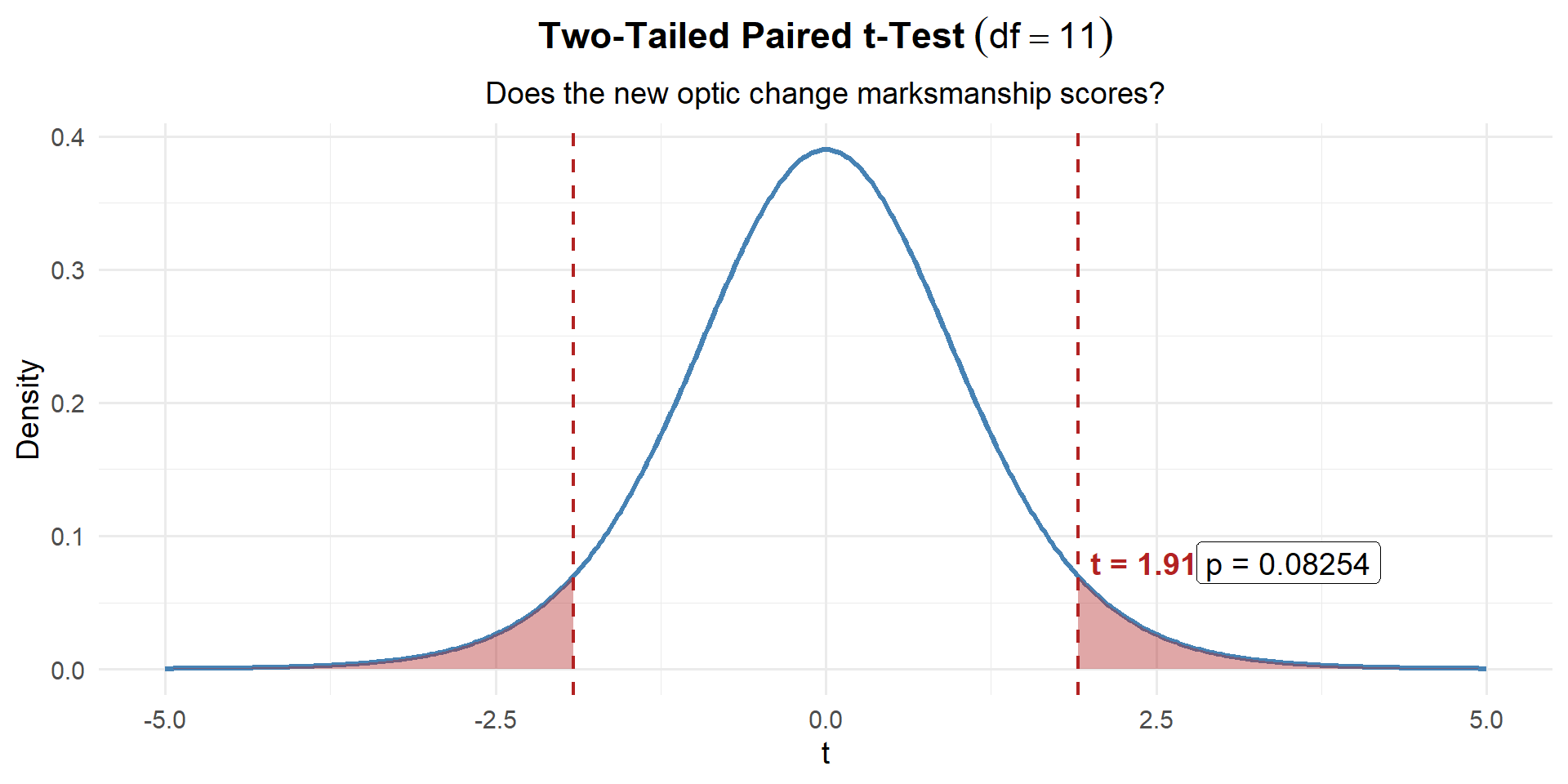
p_value <- 2 * (1 - pt(abs(t_stat), df = n - 1))
p_value
[1] 0.08186423Step 4: Decide and Conclude
\(p = 0.0819 > 0.05\). We fail to reject \(H_0\). At the 5% significance level, there is not sufficient evidence that the new optic changes marksmanship scores. The PSG does not have enough evidence to justify the switch.
Confidence Interval for the Mean Difference
\[\bar{d} \pm t_{\alpha/2, \, n-1} \cdot \frac{s_d}{\sqrt{n}}\]
t_crit <- qt(0.975, df = n - 1)
me <- t_crit * s_d / sqrt(n)
c(d_bar - me, d_bar + me)
[1] -0.1120703 1.6120703We are 95% confident that the true average change in marksmanship score is between -0.11 and 1.61 points.
Since the interval contains zero, this is consistent with failing to reject \(H_0\).
The Inference Toolkit
NoteSummary of Confidence Intervals
| One-Sample Mean (Large) | One-Sample Mean (Small) | One Proportion | Two-Sample Mean | Paired Mean | |
|---|---|---|---|---|---|
| Parameter | \(\mu\) | \(\mu\) | \(p\) | \(\mu_1 - \mu_2\) | \(\mu_d\) |
| Formula | \(\bar{x} \pm z_{\alpha/2} \cdot \dfrac{\sigma}{\sqrt{n}}\) | \(\bar{x} \pm t_{\alpha/2,\, n-1} \cdot \dfrac{s}{\sqrt{n}}\) | \(\hat{p} \pm z_{\alpha/2} \cdot \sqrt{\dfrac{\hat{p}(1-\hat{p})}{n}}\) | \((\bar{x}_1 - \bar{x}_2) \pm t_{\alpha/2} \cdot \sqrt{\dfrac{s_1^2}{n_1} + \dfrac{s_2^2}{n_2}}\) | \(\bar{d} \pm t_{\alpha/2,\, n-1} \cdot \dfrac{s_d}{\sqrt{n}}\) |
| Conditions | \(n \geq 30\) | Normal pop or \(n \geq 30\) | \(n\hat{p} \geq 10\) & \(n(1-\hat{p}) \geq 10\) | \(n_1, n_2 \geq 30\) (or Normal pops) | Diffs ~ Normal or \(n \geq 30\) |
NoteSummary of Hypothesis Tests
| One-Sample Mean (Large) | One-Sample Mean (Small) | One Proportion | Two-Sample Mean (Large) | Two-Sample Mean (Small) | Paired Mean | |
|---|---|---|---|---|---|---|
| Parameter | \(\mu\) | \(\mu\) | \(p\) | \(\mu_1 - \mu_2\) | \(\mu_1 - \mu_2\) | \(\mu_d\) |
| \(H_0\) | \(\mu = \mu_0\) | \(\mu = \mu_0\) | \(p = p_0\) | \(\mu_1 - \mu_2 = \Delta_0\) | \(\mu_1 - \mu_2 = \Delta_0\) | \(\mu_d = \Delta_0\) |
| \(H_a\) | \(\mu \neq, <, > \mu_0\) | \(\mu \neq, <, > \mu_0\) | \(p \neq, <, > p_0\) | \(\mu_1 - \mu_2 \neq, <, > 0\) | \(\mu_1 - \mu_2 \neq, <, > 0\) | \(\mu_d \neq, <, > 0\) |
| Test Statistic | \(z = \dfrac{\bar{x} - \mu_0}{\sigma / \sqrt{n}}\) | \(t = \dfrac{\bar{x} - \mu_0}{s / \sqrt{n}}\) | \(z = \dfrac{\hat{p} - p_0}{\sqrt{p_0(1-p_0)/n}}\) | \(z = \dfrac{\bar{x}_1 - \bar{x}_2}{\sqrt{s_1^2/n_1 + s_2^2/n_2}}\) | \(t = \dfrac{\bar{x}_1 - \bar{x}_2}{\sqrt{s_1^2/n_1 + s_2^2/n_2}}\) | \(t = \dfrac{\bar{d} - \Delta_0}{s_d / \sqrt{n}}\) |
| Distribution | \(N(0,1)\) | \(t_{n-1}\) | \(N(0,1)\) | \(N(0,1)\) | \(t_{df}\) | \(t_{n-1}\) |
| Left-tailed \(p\)-value | pnorm(z) |
pt(t, df=n-1) |
pnorm(z) |
pnorm(z) |
pt(t, df) |
pt(t, df=n-1) |
| Right-tailed \(p\)-value | 1 - pnorm(z) |
1 - pt(t, df=n-1) |
1 - pnorm(z) |
1 - pnorm(z) |
1 - pt(t, df) |
1 - pt(t, df=n-1) |
| Two-tailed \(p\)-value | 2*(1 - pnorm(abs(z))) |
2*(1 - pt(abs(t), df=n-1)) |
2*(1 - pnorm(abs(z))) |
2*(1 - pnorm(abs(z))) |
2*(1 - pt(abs(t), df)) |
2*(1 - pt(abs(t), df=n-1)) |
| Conditions | \(n \geq 30\) | Normal pop or \(n \geq 30\) | \(np_0 \geq 10\) & \(n(1-p_0) \geq 10\) | \(n_1, n_2 \geq 30\) | Populations ~ Normal | Diffs ~ Normal or \(n \geq 30\) |
Decision rule is always the same: \(p \leq \alpha\) → Reject \(H_0\). \(p > \alpha\) → Fail to reject \(H_0\).
Off to Vantage!
Now we’re going to log into Army Vantage and learn how to use R’s t.test() function to run these tests on real data. Have your CAC ready.
Board Problems
Problem 2: Paired or Not-Paired?
For each scenario, state whether the data are paired or not-paired.
NoteQuestions
40 cadets from 1st Regiment vs. 45 cadets from 2nd Regiment compare AFT scores.
30 patients have blood pressure measured before and 1 hour after taking a new medication.
A study compares test scores of 20 students who used a study app vs. 20 who did not.
Each of 15 Soldiers fires a qualification course with iron sights, then again with an optic.
First-born twins’ GPA compared to second-born twins’ GPA for 25 pairs.
TipAnswers
Not-paired. Different cadets in each group.
Paired. Same patients before and after — each patient is their own control.
Not-paired. Different students in each group.
Paired. Same Soldiers fire under both conditions.
Paired. Each twin pair creates a natural match.
Problem 3: Screen Time Reduction
A wellness program claims to reduce cadets’ daily screen time. 20 cadets report average daily screen time (hours) before and after a 4-week program. Summary statistics for the differences (Before \(-\) After):
| \(n\) | \(\bar{d}\) | \(s_d\) | |
|---|---|---|---|
| 20 | 0.8 | 1.5 |
NoteQuestions
State the hypotheses.
Compute the test statistic and \(p\)-value.
At \(\alpha = 0.05\), state your conclusion in context.
Construct a 95% CI for \(\mu_d\). Does it support the test result?
TipAnswers
\(H_0: \mu_d = 0\) vs. \(H_a: \mu_d > 0\) (screen time decreased)
n <- 20; d_bar <- 0.8; s_d <- 1.5
t_stat <- d_bar / (s_d / sqrt(n))
t_stat[1] 2.385139p_value <- 1 - pt(t_stat, df = n - 1)
p_value[1] 0.01382281\(p = 0.0138 \leq 0.05\), so we reject \(H_0\). At the 5% significance level, there is sufficient evidence that the wellness program reduced daily screen time.
t_crit <- qt(0.975, df = n - 1)
me <- t_crit * s_d / sqrt(n)
c(d_bar - me, d_bar + me)
[1] 0.09797839 1.50202161We are 95% confident that the true average screen time reduction is between 0.1 and 1.5 hours per day. The entire interval is above 0, consistent with rejecting \(H_0\).
Problem 4: Ruck March Pace
A platoon sergeant records ruck march completion times (minutes) for 12 Soldiers on two routes of equal distance — one flat, one hilly:
| \(n\) | \(\bar{d}\) (Hilly \(-\) Flat) | \(s_d\) | |
|---|---|---|---|
| 12 | 8.3 | 5.1 |
NoteQuestions
Is this paired or not-paired? Why?
Test whether the hilly route takes significantly longer at \(\alpha = 0.05\).
Construct a 90% CI for \(\mu_d\) and interpret.
TipAnswers
Paired. The same 12 Soldiers complete both routes — each Soldier is measured twice.
\(H_0: \mu_d = 0\) vs. \(H_a: \mu_d > 0\) (hilly takes longer)
n <- 12; d_bar <- 8.3; s_d <- 5.1
t_stat <- d_bar / (s_d / sqrt(n))
t_stat
[1] 5.637656p_value <- 1 - pt(t_stat, df = n - 1)
p_value[1] 7.578481e-05\(p = 1e-04 \leq 0.05\), so we reject \(H_0\). At the 5% significance level, there is sufficient evidence that the hilly route takes significantly longer. The average difference was 8.3 minutes.
t_crit <- qt(0.95, df = n - 1)  # 90% CI
me <- t_crit * s_d / sqrt(n)
c(d_bar - me, d_bar + me)
[1] 5.656021 10.943979We are 90% confident that the true average time difference (hilly minus flat) is between 5.66 and 10.94 minutes.
Before You Leave
Today
- Paired data: Same subjects measured twice → compute differences → one-sample \(t\)-test
- Key formula: \(t = \dfrac{\bar{d}}{s_d / \sqrt{n}}\) with \(df = n - 1\)
- CI for \(\mu_d\): \(\bar{d} \pm t_{\alpha/2, n-1} \cdot \dfrac{s_d}{\sqrt{n}}\)
- Pairing removes between-subject variability — more power to detect real effects
- Ask: “Are these the same subjects measured twice?” → If yes, pair.
Any questions?
Next Lesson
Lesson 25: Two Population Proportions
- Check large-sample conditions for two proportions
- Test \(p_1 - p_2\) using pooled SE
- Construct and interpret a CI for \(p_1 - p_2\)
Upcoming Graded Events
- WebAssign 9.3 - Due before Lesson 25
- WPR II - Lesson 27