Lesson 12: Continuous Random Variables
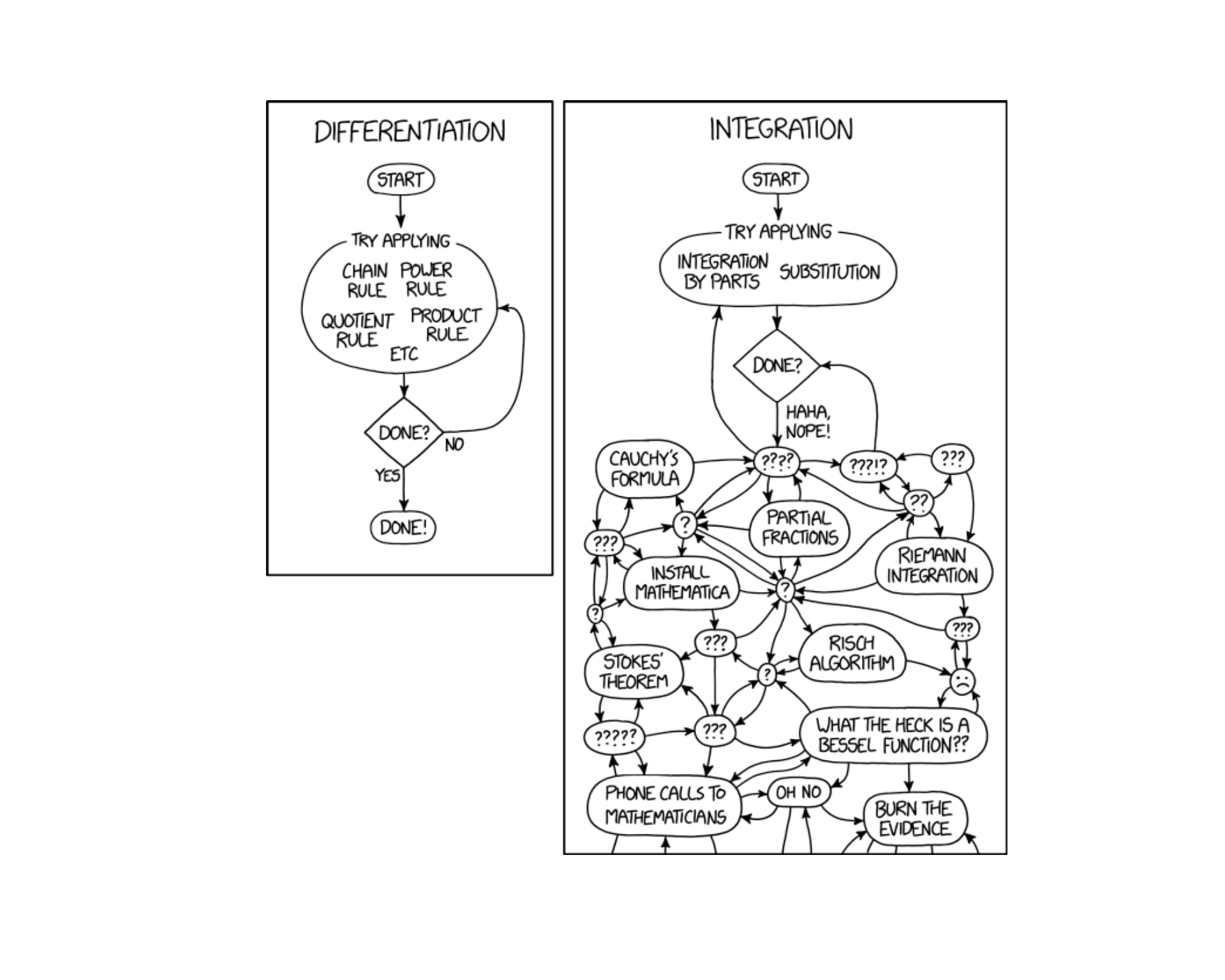
Today we start computing probabilities by integrating PDFs. As this comic shows, differentiation is mechanics — integration is art. The good news: most of our integrals today are just rectangles and triangles.
What We Did: Lessons 6–11
NoteReview: Lessons 6–11
NoteLesson 6: Probability Basics
Sample Spaces and Events:
- Sample space \(S\) = set of all possible outcomes
- Event = subset of the sample space
- Operations: Union (\(A \cup B\)), Intersection (\(A \cap B\)), Complement (\(A^c\))
Kolmogorov Axioms:
- \(P(A) \geq 0\)
- \(P(S) = 1\)
- For mutually exclusive events: \(P(A \cup B) = P(A) + P(B)\)
Key Rules:
- Complement Rule: \(P(A^c) = 1 - P(A)\)
- Addition Rule: \(P(A \cup B) = P(A) + P(B) - P(A \cap B)\)
NoteLesson 7: Conditional Probability
Conditional Probability: \[P(A \mid B) = \frac{P(A \cap B)}{P(B)}\]
Multiplication Rule: \[P(A \cap B) = P(A) \cdot P(B \mid A) = P(B) \cdot P(A \mid B)\]
Law of Total Probability: \[P(A) = P(B) \cdot P(A \mid B) + P(B^c) \cdot P(A \mid B^c)\]
Bayes’ Theorem: \[P(B \mid A) = \frac{P(B) \cdot P(A \mid B)}{P(B) \cdot P(A \mid B) + P(B^c) \cdot P(A \mid B^c)}\]
NoteLesson 8: Counting & Independence
Counting Formulas:
| With Replacement | Without Replacement | |
|---|---|---|
| Ordered | \(n^k\) | \(P(n,k) = \frac{n!}{(n-k)!}\) |
| Unordered | \(\binom{n+k-1}{k}\) | \(\binom{n}{k} = \frac{n!}{k!(n-k)!}\) |
Independence:
- \(A\) and \(B\) are independent if \(P(A \cap B) = P(A) \cdot P(B)\)
- Equivalently: \(P(A \mid B) = P(A)\)
- Independent \(\neq\) Mutually Exclusive!
NoteLesson 9: Discrete Random Variables
Random Variables:
- A random variable \(X\) assigns a numerical value to each outcome in a sample space
- Discrete RVs take finite or countably infinite values
PMF: \(p(x) = P(X = x)\) with \(p(x) \geq 0\) and \(\sum p(x) = 1\)
CDF: \(F(x) = P(X \leq x) = \sum_{y \leq x} p(y)\)
Expected Value: \(E(X) = \sum x \cdot p(x)\)
Variance: \(Var(X) = \sum (x - \mu)^2 \cdot p(x) = E(X^2) - [E(X)]^2\)
NoteLesson 10: Binomial Distribution
BINS Conditions:
- Binary outcomes (success/failure)
- Independent trials
- Number of trials is fixed (\(n\))
- Same probability (\(p\)) each trial
Key Formulas: If \(X \sim \text{Binomial}(n, p)\):
- PMF: \(P(X = x) = \binom{n}{x} p^x (1-p)^{n-x}\)
- Mean: \(E(X) = np\)
- Variance: \(Var(X) = np(1-p)\)
R Functions: dbinom(x, size, prob) for PMF, pbinom(x, size, prob) for CDF
NoteLesson 11: Poisson Distribution
When to Use Poisson:
- Counting events in a fixed interval (time, area, volume)
- Events occur independently at a constant average rate \(\lambda\)
Key Formulas: If \(X \sim \text{Poisson}(\lambda)\):
- PMF: \(P(X = x) = \frac{e^{-\lambda} \lambda^x}{x!}, \quad x = 0, 1, 2, \ldots\)
- Mean: \(E(X) = \lambda\)
- Variance: \(Var(X) = \lambda\)
R Functions: dpois(x, lambda) for PMF, ppois(x, lambda) for CDF
What We’re Doing: Lesson 12
Objectives
- Interpret PDFs and areas as probabilities
- Compute probabilities from PDFs and CDFs
- Find \(E(X)\) and \(Var(X)\) for continuous random variables
Required Reading
Devore, Sections 4.1, 4.2
Break!
Reese
Cal
DMath Basketball!!
Math vs Garrison
NotePreviously 8-2
8-3

Math vs Garrison
NotePreviously 8-3
8-4
Army


SSG Michael Ollis — Medal of Honor (posthumous)
10th Mountain Division, 2-22 IN — KIA 28 Aug 2013, Afghanistan
Shielded a Polish officer from a suicide bomber, sacrificing his life.
The Takeaway for Today
NoteKey Concepts: Continuous Random Variables
Continuous vs. Discrete:
- Discrete RVs: probabilities come from a PMF — \(P(X = x)\)
- Continuous RVs: probabilities come from areas under a PDF — \(P(a \leq X \leq b) = \int_a^b f(x)\,dx\)
Probability Density Function (PDF): \(f(x)\) where:
- \(f(x) \geq 0\) for all \(x\)
- \(\int_{-\infty}^{\infty} f(x)\,dx = 1\)
- \(P(a \leq X \leq b) = \int_a^b f(x)\,dx\)
Cumulative Distribution Function (CDF): \[F(x) = P(X \leq x) = \int_{-\infty}^{x} f(t)\,dt\]
Expected Value and Variance:
- \(E(X) = \int_{-\infty}^{\infty} x \cdot f(x)\,dx\)
- \(Var(X) = \int_{-\infty}^{\infty} (x - \mu)^2 \cdot f(x)\,dx = E(X^2) - [E(X)]^2\)
Critical Difference: For continuous RVs, \(P(X = c) = 0\) for any single value \(c\).
From Discrete to Continuous
The Big Shift
In Lessons 9–11, we worked with discrete random variables — they take on countable values (0, 1, 2, …), and we assign probability to each value using a PMF.
NoteDiscrete Distributions We Know
| General Discrete | Binomial | Poisson | |
|---|---|---|---|
| Notation | \(X\) with PMF table | \(X \sim \text{Binomial}(n, p)\) | \(X \sim \text{Poisson}(\lambda)\) |
| Use when | Any discrete setting | Fixed \(n\) trials, counting successes | Fixed interval, counting events |
| Parameters | Given by PMF table | \(n\) = trials, \(p\) = success probability | \(\lambda\) = average rate |
| PMF | \(p(x) = P(X = x)\) | \(P(X=x) = \binom{n}{x}p^x(1-p)^{n-x}\) | \(P(X=x) = \frac{e^{-\lambda}\lambda^x}{x!}\) |
| Support | Specified by problem | \(x = 0, 1, 2, \ldots, n\) | \(x = 0, 1, 2, \ldots\) |
| Mean | \(\mu = \sum x \cdot p(x)\) | \(\mu = np\) | \(\mu = \lambda\) |
| Variance | \(\sigma^2 = \sum(x-\mu)^2 p(x)\) | \(\sigma^2 = np(1-p)\) | \(\sigma^2 = \lambda\) |
| R PMF | Manual / table lookup | dbinom(x, size, prob) |
dpois(x, lambda) |
| R CDF | cumsum() on PMF |
pbinom(x, size, prob) |
ppois(x, lambda) |
But many quantities in the real world are continuous:
- Time until a piece of equipment fails
- Weight of ammunition in a crate
- Distance a mortar round travels
- Body temperature of a soldier
For these, \(X\) can take any value in an interval. There are infinitely (uncountably!) many possible values, so we can’t assign probability to each one individually.
Discrete vs. Continuous Random Variables
| Discrete | Continuous | |
|---|---|---|
| Values | Countable (0, 1, 2, …) | Any value in an interval |
| Examples | Number of heads, number of breakdowns | Time, weight, distance, temperature |
| How many possible values? | Finite or countably infinite | Uncountably infinite |
| Can you list all values? | Yes | No |
Probability Density Functions (PDFs)
What is a PDF?
NoteRecall: Probability Mass Function (PMF): Discrete
A PMF \(p(x)\) for a discrete random variable \(X\) satisfies:
- \(p(x) \geq 0\) for all \(x\)
- \(\sum_{\text{all } x} p(x) = 1\) (all probabilities sum to 1)
Probabilities are computed by summing:
\[P(a \leq X \leq b) = \sum_{x=a}^{b} p(x)\]
ImportantProbability Density Function (PDF): Continuous
A probability density function \(f(x)\) for a continuous random variable \(X\) satisfies:
- \(f(x) \geq 0\) for all \(x\)
- \(\int_{-\infty}^{\infty} f(x)\,dx = 1\) (total area under the curve equals 1)
Probabilities are computed as areas under the curve:
\[P(a \leq X \leq b) = \int_a^b f(x)\,dx\]
The structure is the same — non-negative, totals to 1, use it to find probabilities over a range. The difference: sums become integrals.
Example
Consider a continuous random variable \(X\) with PDF:
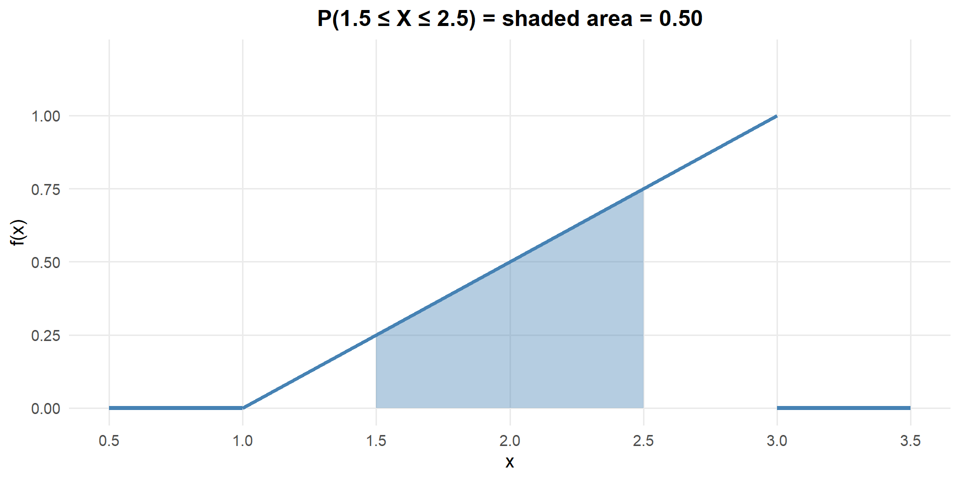
\[f(x) = \begin{cases} \frac{x-1}{2} & 1 \leq x \leq 3 \\ 0 & \text{otherwise} \end{cases}\]
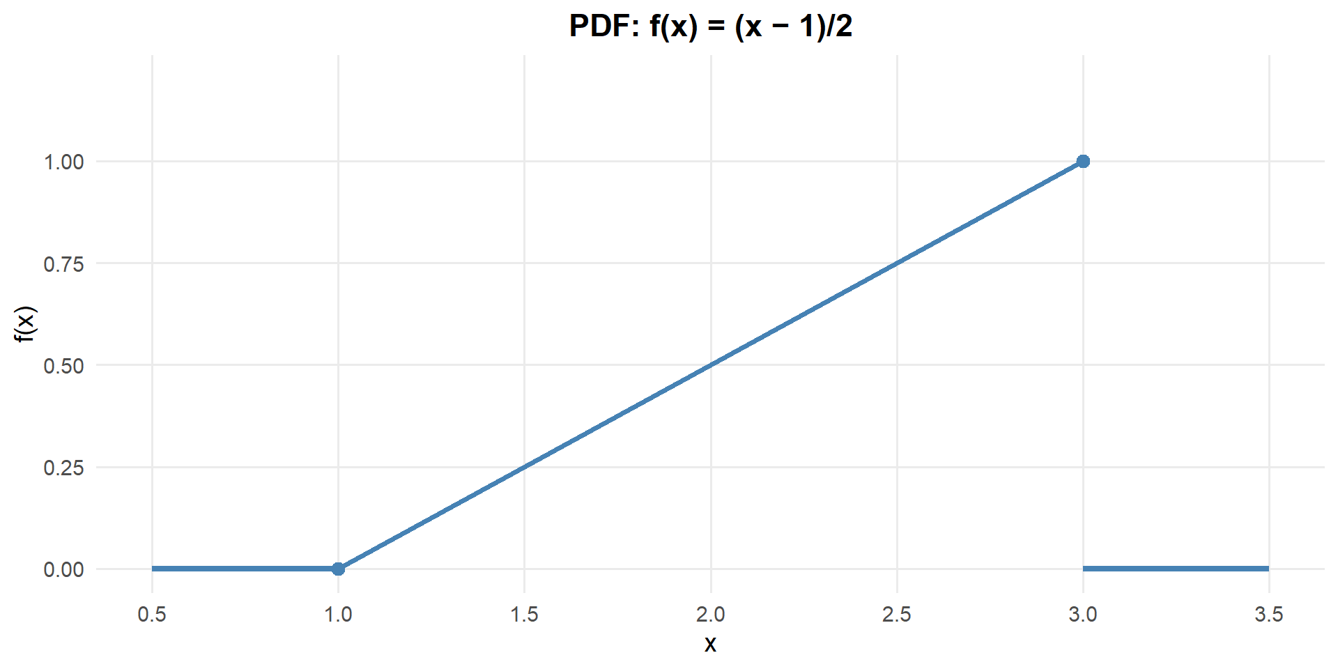
Notice this PDF has a slope — larger values of \(x\) have higher density. The density increases linearly from 0 at \(x = 1\) to 1 at \(x = 3\).
Is this a valid PDF?
For \(f(x)\) to be a valid PDF, we need two things:
\(f(x) \geq 0\) for all \(x\)? Yes — \(\frac{x-1}{2} \geq 0\) on \([1, 3]\).
Total area = 1?
\[\int_1^3 \frac{x-1}{2}\,dx = \frac{(x-1)^2}{4}\Bigg|_1^3 = \frac{4}{4} - \frac{0}{4} = 1 \quad \checkmark\]
You can also see this geometrically: it’s a triangle with base = 2 and height = 1, so area = \(\frac{1}{2}(2)(1) = 1\). ✓
What is \(P(X \leq 2)\)?
\[P(X \leq 2) = \int_1^2 \frac{x-1}{2}\,dx = \frac{(x-1)^2}{4}\Bigg|_1^2 = \frac{1}{4} - 0 = 0.25\]
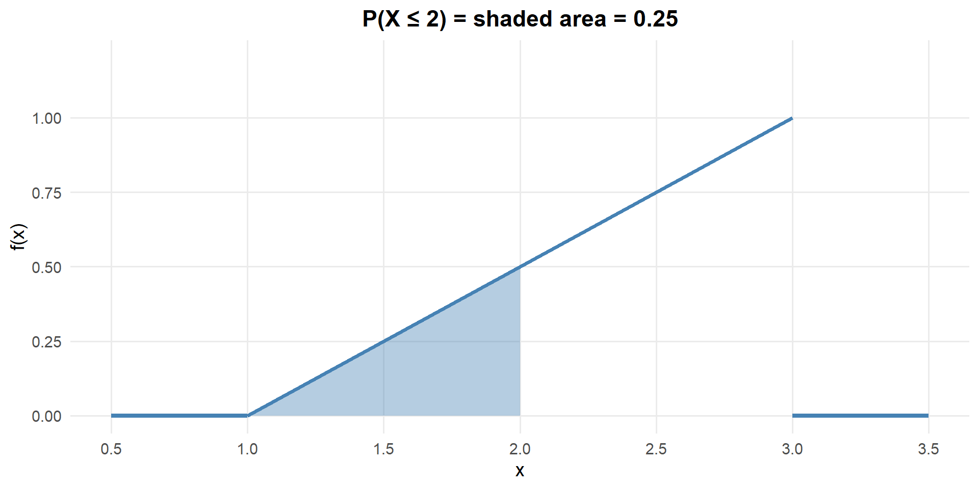
Only 25% of the probability is below \(x = 2\) — makes sense since the PDF is low for small \(x\).
What is \(P(1.5 \leq X \leq 2.5)\)?
\[P(1.5 \leq X \leq 2.5) = \int_{1.5}^{2.5} \frac{x-1}{2}\,dx = \frac{(x-1)^2}{4}\Bigg|_{1.5}^{2.5} = \frac{2.25}{4} - \frac{0.25}{4} = \frac{2}{4} = 0.50\]
What is \(P(X = 2)\)?
\[P(X = 2) = \int_2^2 \frac{x-1}{2}\,dx = 0\]
ImportantA Critical Fact
For any continuous random variable:
\[P(X = c) = \int_c^c f(x)\,dx = 0\]
The “area” under a curve at a single point is zero.
Practical consequence:
\[P(a \leq X \leq b) = P(a < X < b) = P(a \leq X < b) = P(a < X \leq b)\]
It doesn’t matter whether we include the endpoints — the probability is the same!
This is very different from discrete RVs, where \(P(X = x)\) can be large. For continuous RVs, probability only accumulates over intervals.
The Cumulative Distribution Function (CDF)
CDF for Continuous RVs
ImportantCumulative Distribution Function
The CDF of a continuous random variable \(X\) with PDF \(f(x)\) is:
\[F(x) = P(X \leq x) = \int_{-\infty}^{x} f(t)\,dt\]
Properties:
- \(F(x)\) is non-decreasing
- \(\lim_{x \to -\infty} F(x) = 0\) and \(\lim_{x \to \infty} F(x) = 1\)
- \(P(a \leq X \leq b) = F(b) - F(a)\)
- \(f(x) = F'(x)\) — the PDF is the derivative of the CDF
CDF of Our Example
For our PDF \(f(x) = \frac{x-1}{2}\) on \([1, 3]\):
\[F(x) = \int_1^x \frac{t-1}{2}\,dt = \frac{(t-1)^2}{4}\Bigg|_1^x = \frac{(x-1)^2}{4} - \frac{(1-1)^2}{4} = \frac{(x-1)^2}{4}\]
So:
\[F(x) = \begin{cases} 0 & x < 1 \\ \frac{(x-1)^2}{4} & 1 \leq x \leq 3 \\ 1 & x > 3 \end{cases}\]
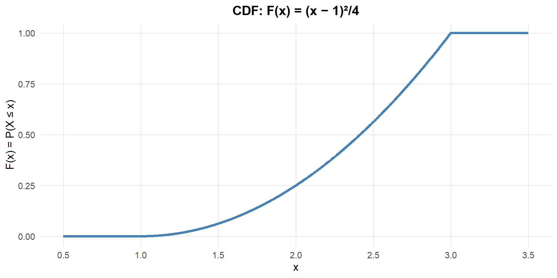
Notice the CDF is a curve (not a straight line) because the PDF has a slope. The CDF accelerates — probability accumulates faster as \(x\) increases because the PDF is taller there.
Our CDF:
\[F(x) = \begin{cases} 0 & x < 1 \\ \frac{(x-1)^2}{4} & 1 \leq x \leq 3 \\ 1 & x > 3 \end{cases}\]
What is \(P(X \leq 2)\)?
\[F(2) = \frac{(2-1)^2}{4} = \frac{1}{4} = 0.25\]
Same answer as before — the CDF just gives it to us directly without re-integrating!
What is \(P(1.5 \leq X \leq 2.5)\)?
\[P(1.5 \leq X \leq 2.5) = F(2.5) - F(1.5) = \frac{(2.5-1)^2}{4} - \frac{(1.5-1)^2}{4} = \frac{2.25}{4} - \frac{0.25}{4} = 0.50\]
Again, same answer — but using the CDF is often easier than re-doing the integral from scratch.
What is \(P(X = 2)\)?
\[P(X = 2) = F(2) - F(2) = 0\]
Still zero! The CDF confirms what we already know: for continuous RVs, the probability at a single point is always zero.
What is \(P(X > 2)\)?
\[P(X > 2) = 1 - F(2) = 1 - \frac{1}{4} = 0.75\]
75% of the probability is above \(x = 2\) — consistent with what we see in the PDF (most of the area is to the right).
Expected Value and Variance
Same concepts as discrete — just replace sums (\(\sum\)) with integrals (\(\int\)):
NoteDiscrete vs Continuous Formulas
| Discrete | Continuous | |
|---|---|---|
| Mean | \(E(X) = \sum x \cdot p(x)\) | \(E(X) = \int x \cdot f(x)\,dx\) |
| Variance | \(Var(X) = \sum (x-\mu)^2 \cdot p(x)\) | \(Var(X) = \int (x-\mu)^2 \cdot f(x)\,dx\) |
| Shortcut | \(Var(X) = E(X^2) - [E(X)]^2\) | \(Var(X) = E(X^2) - [E(X)]^2\) |
| SD | \(\sigma = \sqrt{Var(X)}\) | \(\sigma = \sqrt{Var(X)}\) |
Back to Our Example
Recall our PDF: \(f(x) = \frac{x-1}{2}\) on \([1, 3]\).
What is \(E(X)\)?
\[E(X) = \int_1^3 x \cdot \frac{x-1}{2}\,dx = \int_1^3 \frac{x^2 - x}{2}\,dx\]
\[= \frac{1}{2}\left[\frac{x^3}{3} - \frac{x^2}{2}\right]_1^3 = \frac{1}{2}\left[\left(\frac{27}{3} - \frac{9}{2}\right) - \left(\frac{1}{3} - \frac{1}{2}\right)\right]\]
\[= \frac{1}{2}\left[\left(9 - 4.5\right) - \left(0.333 - 0.5\right)\right] = \frac{1}{2}\left[4.5 + 0.167\right] = \frac{1}{2}\left[\frac{14}{3}\right] = \frac{7}{3} \approx 2.333\]
The mean is \(\frac{7}{3} \approx 2.33\) — shifted toward the right, which makes sense because the PDF puts more weight on larger values of \(x\).
What is \(Var(X)\)?
Using the shortcut \(Var(X) = E(X^2) - [E(X)]^2\):
Step 1: Find \(E(X^2)\):
\[E(X^2) = \int_1^3 x^2 \cdot \frac{x-1}{2}\,dx = \int_1^3 \frac{x^3 - x^2}{2}\,dx\]
\[= \frac{1}{2}\left[\frac{x^4}{4} - \frac{x^3}{3}\right]_1^3 = \frac{1}{2}\left[\left(\frac{81}{4} - \frac{27}{3}\right) - \left(\frac{1}{4} - \frac{1}{3}\right)\right]\]
\[= \frac{1}{2}\left[\left(20.25 - 9\right) - \left(0.25 - 0.333\right)\right] = \frac{1}{2}\left[11.25 + 0.083\right] = \frac{1}{2} \cdot \frac{34}{3} = \frac{17}{3} \approx 5.667\]
Step 2: Apply the shortcut:
\[Var(X) = E(X^2) - [E(X)]^2 = \frac{17}{3} - \left(\frac{7}{3}\right)^2 = \frac{17}{3} - \frac{49}{9} = \frac{51}{9} - \frac{49}{9} = \frac{2}{9} \approx 0.222\]
What is \(SD(X)\)?
\[SD(X) = \sqrt{Var(X)} = \sqrt{\frac{2}{9}} = \frac{\sqrt{2}}{3} \approx 0.471\]
Board Problems
Problem 1
A continuous random variable \(X\) has the following PDF:
\[f(x) = \begin{cases} kx^2 & 0 \leq x \leq 3 \\ 0 & \text{otherwise} \end{cases}\]
NoteQuestions
Find the value of \(k\) that makes \(f(x)\) a valid PDF.
Find the CDF \(F(x)\).
What is \(P(X = 2)\)?
What is \(P(X < 1)\)?
What is \(P(X > 2)\)?
What is \(P(1 \leq X \leq 2)\)?
Find \(E(X)\) and \(Var(X)\).
What is the probability that \(X\) is more than 2 standard deviations above the mean?
TipAnswers
- We need \(\int_0^3 kx^2\,dx = 1\):
\[k \cdot \frac{x^3}{3}\Big|_0^3 = k \cdot \frac{27}{3} = 9k = 1 \implies k = \frac{1}{9}\]
So \(f(x) = \frac{x^2}{9}\) on \([0, 3]\).
- For \(0 \leq x \leq 3\):
\[F(x) = \int_0^x \frac{t^2}{9}\,dt = \frac{t^3}{27}\Big|_0^x = \frac{x^3}{27}\]
So: \(F(x) = \begin{cases} 0 & x < 0 \\ x^3/27 & 0 \leq x \leq 3 \\ 1 & x > 3 \end{cases}\)
\(P(X = 2) = 0\) — for any continuous random variable, the probability of any single exact value is 0.
\(P(X < 1) = F(1) = \frac{1^3}{27} = \frac{1}{27} \approx 0.037\)
\(P(X > 2) = 1 - F(2) = 1 - \frac{8}{27} = \frac{19}{27} \approx 0.704\)
\(P(1 \leq X \leq 2) = F(2) - F(1) = \frac{8}{27} - \frac{1}{27} = \frac{7}{27} \approx 0.259\)
\(E(X) = \int_0^3 x \cdot \frac{x^2}{9}\,dx = \int_0^3 \frac{x^3}{9}\,dx = \frac{x^4}{36}\Big|_0^3 = \frac{81}{36} = \frac{9}{4} = 2.25\)
\(E(X^2) = \int_0^3 x^2 \cdot \frac{x^2}{9}\,dx = \int_0^3 \frac{x^4}{9}\,dx = \frac{x^5}{45}\Big|_0^3 = \frac{243}{45} = \frac{27}{5} = 5.4\)
\(Var(X) = E(X^2) - [E(X)]^2 = 5.4 - (2.25)^2 = 5.4 - 5.0625 = 0.3375\)
\(SD(X) = \sqrt{0.3375} \approx 0.581\)
- 2 standard deviations above the mean: \(\mu + 2\sigma = 2.25 + 2(0.581) = 3.412\)
Since \(3.412 > 3\) and the PDF is only defined on \([0, 3]\), we have \(P(X > 3.412) = 0\).
The probability of being more than 2 standard deviations above the mean is 0.
Problem 2: Sentry Duty Wait Time
A sentry expects a supply truck sometime during their 4-hour shift. The truck is equally likely to arrive at any point during the shift. Let \(X\) = time (in hours) until the truck arrives, with PDF:
\[f(x) = \begin{cases} \frac{1}{4} & 0 \leq x \leq 4 \\ 0 & \text{otherwise} \end{cases}\]
NoteQuestions
Verify this is a valid PDF.
What is \(P(X \leq 1)\) — the truck arrives in the first hour?
What is \(P(1 \leq X \leq 3)\)?
Find \(E(X)\) and \(SD(X)\).
The sentry gets relieved early at hour 3. What is the probability the truck has already arrived?
What is the probability the truck arrives in the last 30 minutes of the shift?
TipAnswers
\(\int_0^4 \frac{1}{4}\,dx = \frac{x}{4}\Big|_0^4 = 1\) ✓
\(P(X \leq 1) = \int_0^1 \frac{1}{4}\,dx = \frac{1}{4} = 0.25\)
\(P(1 \leq X \leq 3) = \int_1^3 \frac{1}{4}\,dx = \frac{2}{4} = 0.50\)
\(E(X) = \int_0^4 x \cdot \frac{1}{4}\,dx = \frac{x^2}{8}\Big|_0^4 = \frac{16}{8} = 2\) hours
\(E(X^2) = \int_0^4 x^2 \cdot \frac{1}{4}\,dx = \frac{x^3}{12}\Big|_0^4 = \frac{64}{12} = \frac{16}{3}\)
\(Var(X) = \frac{16}{3} - 4 = \frac{4}{3}\)
\(SD(X) = \sqrt{4/3} \approx 1.155\) hours
\(P(X \leq 3) = \int_0^3 \frac{1}{4}\,dx = \frac{3}{4} = 0.75\)
\(P(3.5 \leq X \leq 4) = \int_{3.5}^4 \frac{1}{4}\,dx = \frac{0.5}{4} = 0.125\)
Problem 3: Fuel Consumption
A tactical vehicle’s fuel consumption rate (gallons per mile) on a certain terrain follows the PDF:
\[f(x) = \begin{cases} 6x(1-x) & 0 \leq x \leq 1 \\ 0 & \text{otherwise} \end{cases}\]
NoteQuestions
Verify this is a valid PDF.
What is the probability the fuel consumption rate is less than 0.5 gallons per mile?
What is the probability the rate is between 0.25 and 0.75?
Find \(E(X)\) — the expected fuel consumption rate.
Find \(Var(X)\) and \(SD(X)\).
Is it more likely that the rate is above or below 0.5? Explain.
TipAnswers
\(\int_0^1 6x(1-x)\,dx = \int_0^1 (6x - 6x^2)\,dx = \left[3x^2 - 2x^3\right]_0^1 = 3 - 2 = 1\) ✓
\(P(X < 0.5) = \int_0^{0.5} 6x(1-x)\,dx = \left[3x^2 - 2x^3\right]_0^{0.5} = 0.75 - 0.25 = 0.50\)
\(P(0.25 \leq X \leq 0.75) = \int_{0.25}^{0.75} 6x(1-x)\,dx = \left[3x^2 - 2x^3\right]_{0.25}^{0.75}\)
\(= (3(0.5625) - 2(0.421875)) - (3(0.0625) - 2(0.015625)) = (1.6875 - 0.84375) - (0.1875 - 0.03125) = 0.84375 - 0.15625 = 0.6875\)
\(E(X) = \int_0^1 x \cdot 6x(1-x)\,dx = \int_0^1 (6x^2 - 6x^3)\,dx = \left[2x^3 - \frac{3x^4}{2}\right]_0^1 = 2 - 1.5 = 0.5\)
\(E(X^2) = \int_0^1 x^2 \cdot 6x(1-x)\,dx = \int_0^1 (6x^3 - 6x^4)\,dx = \left[\frac{3x^4}{2} - \frac{6x^5}{5}\right]_0^1 = 1.5 - 1.2 = 0.3\)
\(Var(X) = 0.3 - 0.25 = 0.05\)
\(SD(X) = \sqrt{0.05} \approx 0.224\)
- Exactly equally likely! The PDF \(f(x) = 6x(1-x)\) is symmetric about \(x = 0.5\), and we showed \(P(X < 0.5) = 0.50\). So \(P(X > 0.5) = 0.50\) as well.
Problem 4: Marksmanship Score
A cadet’s marksmanship score on a standardized assessment follows a continuous distribution with PDF:
\[f(x) = \begin{cases} \frac{1}{40} & 60 \leq x \leq 100 \\ 0 & \text{otherwise} \end{cases}\]
Let \(X\) = the cadet’s score.
NoteQuestions
Verify this is a valid PDF.
What is \(P(X \geq 90)\) — the probability of scoring 90 or above?
What is the probability the score is between 70 and 85?
Find \(E(X)\) and \(SD(X)\).
A score of 80 or above is “Expert.” What percentage of cadets qualify as Expert?
Given that a cadet scored at least 75, what is the probability they scored at least 90? (Hint: use conditional probability with the CDF)
TipAnswers
\(\int_{60}^{100} \frac{1}{40}\,dx = \frac{x}{40}\Big|_{60}^{100} = \frac{100}{40} - \frac{60}{40} = \frac{40}{40} = 1\) ✓
\(P(X \geq 90) = \int_{90}^{100} \frac{1}{40}\,dx = \frac{10}{40} = 0.25\)
\(P(70 \leq X \leq 85) = \int_{70}^{85} \frac{1}{40}\,dx = \frac{15}{40} = 0.375\)
\(E(X) = \int_{60}^{100} x \cdot \frac{1}{40}\,dx = \frac{x^2}{80}\Big|_{60}^{100} = \frac{10000}{80} - \frac{3600}{80} = \frac{6400}{80} = 80\)
\(E(X^2) = \int_{60}^{100} x^2 \cdot \frac{1}{40}\,dx = \frac{x^3}{120}\Big|_{60}^{100} = \frac{1000000}{120} - \frac{216000}{120} = \frac{784000}{120} \approx 6533.33\)
\(Var(X) = 6533.33 - 80^2 = 6533.33 - 6400 = 133.33\)
\(SD(X) = \sqrt{133.33} \approx 11.55\)
\(P(X \geq 80) = \int_{80}^{100} \frac{1}{40}\,dx = \frac{20}{40} = 0.50\) — 50% qualify as Expert.
\(P(X \geq 90 \mid X \geq 75) = \frac{P(X \geq 90)}{P(X \geq 75)} = \frac{10/40}{25/40} = \frac{10}{25} = 0.40\)
Before You Leave
Today
- Continuous RVs have probabilities given by areas under the PDF, not by the PMF
- PDF: \(f(x) \geq 0\) and \(\int f(x)\,dx = 1\) — but \(f(x)\) is density, not probability
- CDF: \(F(x) = P(X \leq x)\) — use it to compute \(P(a \leq X \leq b) = F(b) - F(a)\)
- \(P(X = c) = 0\) for continuous RVs — endpoints don’t matter
- \(E(X)\) and \(Var(X)\) use integrals instead of sums, but the formulas are analogous
Any questions?
Next Lesson
Lesson 13: Normal Distribution
- Standardize and use normal probabilities
- Find normal quantiles for given tail areas
- Assess plausibility using normal models
Upcoming Graded Events
- WebAssign 4.1–4.2 - Due before Lesson 13
- Lesson 15 - Review (Lessons 1–14)
- WPR I - Lesson 16