Lesson 23: Two Sample t-Test

A Note from LTC Turner

I’m sorry I can’t be with you today. Thank you to MAJ Day for stepping in and leading class. You’re in great hands — pay attention and ask good questions!

What We Did: Lessons 17–22

Lesson 17: Central Limit Theorem

The Central Limit Theorem (CLT): If \(X_1, X_2, \ldots, X_n\) are iid with mean \(\mu\) and standard deviation \(\sigma\), then for large \(n\):

\[\bar{X} \sim N\left(\mu, \frac{\sigma^2}{n}\right)\]

Standard Error of the Mean: \(\sigma_{\bar{X}} = \frac{\sigma}{\sqrt{n}}\)

Rule of thumb: \(n \geq 30\) unless the population is already normal.

Lesson 18: Confidence Intervals I

Confidence Interval for a Mean:

	Formula	When to Use
Large sample (\(n \geq 30\))	\(\bar{X} \pm z_{\alpha/2} \cdot \dfrac{\sigma}{\sqrt{n}}\)	Random sample, independence, \(s \approx \sigma\)
Small sample (\(n < 30\))	\(\bar{X} \pm t_{\alpha/2, n-1} \cdot \dfrac{s}{\sqrt{n}}\)	Random sample, independence, population ~ Normal

Key ideas: Higher confidence → wider interval. Larger \(n\) → narrower interval.

Lesson 19: Confidence Intervals II

Confidence Interval for a Proportion:

\[\hat{p} \pm z_{\alpha/2} \cdot \sqrt{\frac{\hat{p}(1-\hat{p})}{n}}\]

Conditions: \(n\hat{p} \geq 10\) and \(n(1-\hat{p}) \geq 10\)

Interpretation: “We are C% confident that [interval] captures the true [parameter in context].” The confidence level describes the method’s long-run success rate, not the probability any single interval is correct.

Lesson 20: Intro to Hypothesis Testing

Every hypothesis test follows four steps:

State hypotheses: \(H_0\) (null — status quo) vs. \(H_a\) (alternative — what we want to show)
Compute a test statistic: How far is our sample result from what \(H_0\) predicts?
Find the \(p\)-value: If \(H_0\) were true, how likely is a result this extreme or more?
Make a decision: If \(p \leq \alpha\), reject \(H_0\). If \(p > \alpha\), fail to reject \(H_0\).

Lesson 21: One Sample t-Test & One-Proportion z-Test

One-sample \(t\)-test for a mean (\(\sigma\) unknown):

\[t = \frac{\bar{x} - \mu_0}{s / \sqrt{n}}, \qquad df = n - 1\]

One-proportion \(z\)-test:

\[z = \frac{\hat{p} - p_0}{\sqrt{\dfrac{p_0(1 - p_0)}{n}}}\]

Conditions for proportions: \(np_0 \geq 10\) and \(n(1-p_0) \geq 10\) (use \(p_0\), not \(\hat{p}\)!)

Lesson 22: Two-Sample z-Test (Large Samples)

Two-sample \(z\)-test for means (\(n_1 \geq 30\) and \(n_2 \geq 30\)):

\[z = \frac{(\bar{x}_1 - \bar{x}_2) - \Delta_0}{\sqrt{\dfrac{s_1^2}{n_1} + \dfrac{s_2^2}{n_2}}}\]

Conditions: Large samples (\(n_1, n_2 \geq 30\)), independent random samples.

CI for \(\mu_1 - \mu_2\): \((\bar{x}_1 - \bar{x}_2) \pm z_{\alpha/2} \cdot SE\)

Since both samples are large, the CLT kicks in and we use the standard normal \(z\) — no degrees of freedom needed.

Review: The Inference Toolkit

Summary of Confidence Intervals

	One-Sample Mean (Large)	One-Sample Mean (Small)	One Proportion	Two-Sample Mean	Paired Mean
Parameter	\(\mu\)	\(\mu\)	\(p\)	\(\mu_1 - \mu_2\)	\(\mu_d\)
Formula	\(\bar{x} \pm z_{\alpha/2} \cdot \dfrac{\sigma}{\sqrt{n}}\)	\(\bar{x} \pm t_{\alpha/2,\, n-1} \cdot \dfrac{s}{\sqrt{n}}\)	\(\hat{p} \pm z_{\alpha/2} \cdot \sqrt{\dfrac{\hat{p}(1-\hat{p})}{n}}\)	\((\bar{x}_1 - \bar{x}_2) \pm z_{\alpha/2} \cdot SE\)	\(\bar{d} \pm t_{\alpha/2,\, n-1} \cdot \dfrac{s_d}{\sqrt{n}}\)
Conditions	\(n \geq 30\)	\(n \leq 30\)	\(n\hat{p} \geq 10\) & \(n(1-\hat{p}) \geq 10\)	\(n_1, n_2 \geq 30\)	Diffs ~ Normal or \(n \geq 30\)

Summary of Hypothesis Tests

	One-Sample Mean (Large)	One-Sample Mean (Small)	One Proportion	Two-Sample Mean (Large)	Two-Sample Mean (Small)	Paired Mean
Parameter	\(\mu\)	\(\mu\)	\(p\)	\(\mu_1 - \mu_2\)	\(\mu_1 - \mu_2\)	\(\mu_d\)
\(H_0\)	\(\mu = \mu_0\)	\(\mu = \mu_0\)	\(p = p_0\)	\(\mu_1 - \mu_2 = \Delta_0\)	\(\mu_1 - \mu_2 = \Delta_0\)	\(\mu_d = \Delta_0\)
\(H_a\)	\(\mu \neq, <, > \mu_0\)	\(\mu \neq, <, > \mu_0\)	\(p \neq, <, > p_0\)	\(\mu_1 - \mu_2 \neq, <, > 0\)	\(\mu_1 - \mu_2 \neq, <, > 0\)	\(\mu_d \neq, <, > 0\)
Test Statistic	\(z = \dfrac{\bar{x} - \mu_0}{\sigma / \sqrt{n}}\)	\(t = \dfrac{\bar{x} - \mu_0}{s / \sqrt{n}}\)	\(z = \dfrac{\hat{p} - p_0}{\sqrt{p_0(1-p_0)/n}}\)	\(z = \dfrac{\bar{x}_1 - \bar{x}_2}{SE}\)	\(t = \dfrac{\bar{x}_1 - \bar{x}_2}{SE}\)	\(t = \dfrac{\bar{d} - \Delta_0}{s_d / \sqrt{n}}\)
Distribution	\(N(0,1)\)	\(t_{n-1}\)	\(N(0,1)\)	\(N(0,1)\)	\(t_{df}\)	\(t_{n-1}\)
Left-tailed \(p\)-value	`pnorm(z)`	`pt(t, df=n-1)`	`pnorm(z)`	`pnorm(z)`	`pt(t, df)`	`pt(t, df=n-1)`
Right-tailed \(p\)-value	`1 - pnorm(z)`	`1 - pt(t, df=n-1)`	`1 - pnorm(z)`	`1 - pnorm(z)`	`1 - pt(t, df)`	`1 - pt(t, df=n-1)`
Two-tailed \(p\)-value	`2*(1 - pnorm(abs(z)))`	`2*(1 - pt(abs(t), df=n-1))`	`2*(1 - pnorm(abs(z)))`	`2*(1 - pnorm(abs(z)))`	`2*(1 - pt(abs(t), df))`	`2*(1 - pt(abs(t), df=n-1))`
Conditions	\(n \geq 30\)	Normal pop or \(n \geq 30\)	\(np_0 \geq 10\) & \(n(1-p_0) \geq 10\)	\(n_1, n_2 \geq 30\)	Populations ~ Normal	Diffs ~ Normal or \(n \geq 30\)

Decision rule is always the same: \(p \leq \alpha\) → Reject \(H_0\). \(p > \alpha\) → Fail to reject \(H_0\).

What We’re Doing: Lesson 23

Objectives

Review the two-sample \(z\)-test for large samples
Test \(\mu_1 - \mu_2\) with small independent samples using the two-sample \(t\)-test
Identify paired versus independent designs
Test a paired mean difference using the paired \(t\)-test

Required Reading

Devore, Sections 9.2, 9.3

Break!

Reese

Cal

The Takeaway for Today

Today’s Key Ideas

Small-sample two-sample \(t\)-test:

\[t = \frac{(\bar{x}_1 - \bar{x}_2) - \Delta_0}{\sqrt{\dfrac{s_1^2}{n_1} + \dfrac{s_2^2}{n_2}}}, \qquad df = \frac{\left(\dfrac{s_1^2}{n_1} + \dfrac{s_2^2}{n_2}\right)^2}{\dfrac{\left(s_1^2/n_1\right)^2}{n_1 - 1} + \dfrac{\left(s_2^2/n_2\right)^2}{n_2 - 1}}\]

Same formula as the large-sample \(z\), but now we use the \(t\)-distribution because small samples mean more uncertainty in our estimate of \(SE\).

Paired \(t\)-test: Compute \(d_i = x_{1i} - x_{2i}\), then it’s just a one-sample \(t\)-test on \(\bar{d}\):

\[t = \frac{\bar{d} - \Delta_0}{s_d / \sqrt{n}}, \qquad df = n - 1\]

The paired \(t\)-test is not a new test — it’s the same one-sample \(t\)-test from Lesson 21, applied to the vector of differences.

Review: The Two-Sample \(z\)-Test (Large Samples)

Last class we learned how to compare two independent group means when both samples are large (\(n_1 \geq 30\), \(n_2 \geq 30\)):

\[z = \frac{(\bar{x}_1 - \bar{x}_2) - \Delta_0}{\sqrt{\dfrac{s_1^2}{n_1} + \dfrac{s_2^2}{n_2}}}\]

where \(\Delta_0\) is the hypothesized difference (usually 0). Because both samples are large, the CLT guarantees the sampling distribution of \(\bar{x}_1 - \bar{x}_2\) is approximately normal, so we use the \(z\)-distribution and pnorm() for \(p\)-values.

But what happens when one or both samples are small?

New Material: The Two-Sample \(t\)-Test (Small Samples)

When sample sizes are small, \(s_1\) and \(s_2\) are less reliable estimates of \(\sigma_1\) and \(\sigma_2\). This extra uncertainty means the \(z\)-distribution is too optimistic — it underestimates how spread out our test statistic really is.

The fix? Use the \(t\)-distribution, which has heavier tails to account for that uncertainty. Same idea as switching from \(z\) to \(t\) for a one-sample test when \(\sigma\) is unknown and \(n\) is small.

Two-Sample t-Test (Small Samples)

Hypotheses:

\(H_0: \mu_1 - \mu_2 = 0\)

\(H_a: \mu_1 - \mu_2 \neq, <, > \ 0\)

Test statistic: (same formula as the large-sample \(z\)!)

\[t = \frac{(\bar{x}_1 - \bar{x}_2) - \Delta_0}{\sqrt{\dfrac{s_1^2}{n_1} + \dfrac{s_2^2}{n_2}}}\]

where \(\Delta_0\) is the hypothesized difference (usually 0).

Degrees of freedom:

\[df = \frac{\left(\dfrac{s_1^2}{n_1} + \dfrac{s_2^2}{n_2}\right)^2}{\dfrac{\left(s_1^2/n_1\right)^2}{n_1 - 1} + \dfrac{\left(s_2^2/n_2\right)^2}{n_2 - 1}}\]

Note: this is not simply \(n_1 + n_2 - 2\). When computing by hand, round down to the nearest integer — this is the conservative choice because a smaller \(df\) gives heavier tails, making it harder to reject \(H_0\). R computes the exact \(df\) for you.

Conditions: Independent random samples, both populations approximately normal (check with histograms/QQ plots).

\(p\)-values: Use pt() with the appropriate \(df\).

When to Use z vs. t

	Large samples (\(n_1, n_2 \geq 30\))	Small samples
Distribution	\(z\) (standard normal)	\(t\) (with \(df\))
\(p\)-values	`pnorm()`	`pt()`
Normality check	Not needed (CLT)	Required

The test statistic formula is identical — the only difference is which distribution you use to find the \(p\)-value.

Example 1: Rifle Cleaning Time

A company XO wants to know if a new rifle cleaning procedure is faster than the standard method. He randomly assigns Soldiers to two groups:

	Standard Method	New Method
\(n\)	12	10
\(\bar{x}\) (min)	28.5	24.3
\(s\)	4.8	3.9

These are small samples, so we use the two-sample \(t\)-test.

Step 1: State the Hypotheses

The XO suspects the new method is faster (lower times):

\[H_0: \mu_1 - \mu_2 = 0 \qquad \text{vs.} \qquad H_a: \mu_1 - \mu_2 > 0\]

where \(\mu_1\) = standard, \(\mu_2\) = new.

Step 2: Compute the Test Statistic

\[t = \frac{(\bar{x}_1 - \bar{x}_2) - \Delta_0}{SE} = \frac{(28.5 - 24.3) - 0}{\sqrt{\dfrac{4.8^2}{12} + \dfrac{3.9^2}{10}}} = \frac{4.2}{\sqrt{1.920 + 1.521}} = \frac{4.2}{1.855} = 2.26\]

n1 <- 12; n2 <- 10
xbar1 <- 28.5; xbar2 <- 24.3
s1 <- 4.8; s2 <- 3.9

se <- sqrt(s1^2 / n1 + s2^2 / n2)
t_stat <- (xbar1 - xbar2) / se
t_stat

[1] 2.264159

Degrees of freedom:

\[df = \frac{\left(\dfrac{s_1^2}{n_1} + \dfrac{s_2^2}{n_2}\right)^2}{\dfrac{\left(s_1^2/n_1\right)^2}{n_1 - 1} + \dfrac{\left(s_2^2/n_2\right)^2}{n_2 - 1}} = \frac{\left(\dfrac{4.8^2}{12} + \dfrac{3.9^2}{10}\right)^2}{\dfrac{\left(4.8^2/12\right)^2}{11} + \dfrac{\left(3.9^2/10\right)^2}{9}} = \frac{(1.920 + 1.521)^2}{\dfrac{1.920^2}{11} + \dfrac{1.521^2}{9}} = \frac{3.441^2}{\dfrac{3.686}{11} + \dfrac{2.314}{9}} = \frac{11.840}{0.335 + 0.257} = 19.99 \implies \lfloor df \rfloor = 19\]

df <- (s1^2/n1 + s2^2/n2)^2 / ((s1^2/n1)^2/(n1-1) + (s2^2/n2)^2/(n2-1))
df

[1] 19.99486

Step 3: Find the \(p\)-Value

Right-tailed with \(df = 19\):

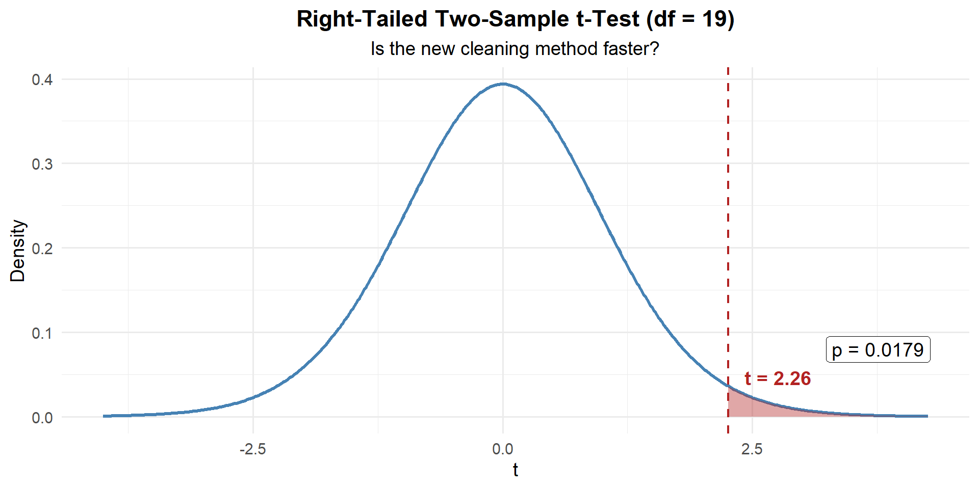
p_value <- 1 - pt(t_stat, df = df)
p_value

[1] 0.01741865

Step 4: Decide and Conclude

\(p = 0.0174 \leq 0.05\). We reject \(H_0\). At the 5% significance level, there is sufficient evidence that the new rifle cleaning method is faster than the standard method. The average time savings was 4.2 minutes.

Example 2: PT Run Times (Small Samples)

A battalion fitness officer wants to compare 2-mile run times between two small units:

	HHC	BSB
\(n\)	15	18
\(\bar{x}\) (min)	15.2	16.1
\(s\)	1.8	2.3

Is there a difference in mean run times?

\[H_0: \mu_1 - \mu_2 = 0 \qquad \text{vs.} \qquad H_a: \mu_1 - \mu_2 \neq 0\]

n1 <- 15; n2 <- 18
xbar1 <- 15.2; xbar2 <- 16.1
s1 <- 1.8; s2 <- 2.3

se <- sqrt(s1^2 / n1 + s2^2 / n2)
t_stat <- (xbar1 - xbar2) / se
df <- (s1^2/n1 + s2^2/n2)^2 / ((s1^2/n1)^2/(n1-1) + (s2^2/n2)^2/(n2-1))
t_stat

[1] -1.260389

df

[1] 30.90224

\[df = \frac{\left(\dfrac{1.8^2}{15} + \dfrac{2.3^2}{18}\right)^2}{\dfrac{\left(1.8^2/15\right)^2}{14} + \dfrac{\left(2.3^2/18\right)^2}{17}} = \frac{\left(0.216 + 0.294\right)^2}{\dfrac{0.216^2}{14} + \dfrac{0.294^2}{17}} = \frac{0.260}{0.00333 + 0.00508} = 30.9 \implies \lfloor df \rfloor = 30\]

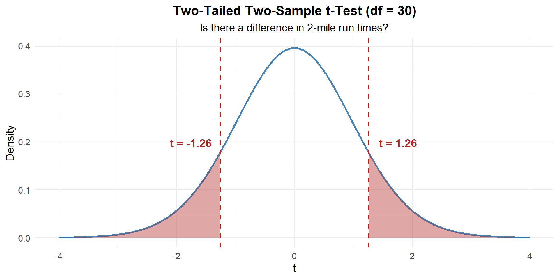
p_value <- 2 * (1 - pt(abs(t_stat), df = df))
p_value

[1] 0.2169634

\(p = 0.217 > 0.05\). We fail to reject \(H_0\). At the 5% significance level, there is not sufficient evidence of a difference in mean 2-mile run times between HHC and BSB.

New Material: The Paired \(t\)-Test

When Are Samples NOT Independent?

So far we’ve compared two separate groups. But sometimes the two “groups” are really the same individuals measured twice:

Same Soldiers’ ACFT scores before and after a training program
Same cadets’ performance on two different tasks
Same rifles tested with old vs. new cleaning method

These are paired observations. The two measurements are not independent — a Soldier who scores high before will probably score high after, too.

The Key Insight: Paired Data → One-Sample Problem

Here’s the beautiful thing about paired data. Once you compute the differences, you’re back to a one-sample problem.

Soldier	Before	After	\(d_i = \text{After} - \text{Before}\)
1	445	460	15
2	478	491	13
3	512	520	8
…	…	…	…

You started with two columns. Now you have one column of differences. And you already know how to do a one-sample \(t\)-test from Lesson 21!

The question “Did scores improve?” becomes “Is the mean of these differences greater than zero?”

The Paired t-Test Is Just a One-Sample t-Test on Differences

Given \(n\) paired observations, define \(d_i = x_{1i} - x_{2i}\).

Now you have a single sample \(d_1, d_2, \ldots, d_n\).

Hypotheses: \(H_0: \mu_d = 0\) vs. \(H_a: \mu_d \neq, <, > \ 0\)

Test statistic: (this IS the one-sample \(t\)-test!)

\[t = \frac{\bar{d} - \Delta_0}{s_d / \sqrt{n}}, \qquad df = n - 1\]

Conditions: Differences are approximately normal (or \(n \geq 30\)).

That’s it. No new formula. No new concept. Just compute differences, then do what you already know.

Why Not Use a Two-Sample Test on Paired Data?

If we ignored the pairing and ran a two-sample test, we’d treat 445 and 460 as if they came from unrelated people. All that natural person-to-person variability would inflate our standard error, making it harder to detect a real effect. Pairing removes between-subject variability and gives us more power.

Example 3: ACFT Scores Before and After a PT Program

A company commander puts 10 Soldiers through a new 6-week PT program:

Soldier	1	2	3	4	5	6	7	8	9	10
Before	445	478	512	390	467	501	423	489	455	438
After	460	491	520	412	475	498	441	502	470	450

Step 1: Compute the differences (this is the key step!)

before <- c(445, 478, 512, 390, 467, 501, 423, 489, 455, 438)
after  <- c(460, 491, 520, 412, 475, 498, 441, 502, 470, 450)
d <- after - before
d

 [1] 15 13  8 22  8 -3 18 13 15 12

Now we have a single vector of numbers. From here it’s a one-sample \(t\)-test.

Step 2: State the Hypotheses

Did scores improve? That means \(\mu_d > 0\):

\[H_0: \mu_d = 0 \qquad \text{vs.} \qquad H_a: \mu_d > 0\]

Step 3: Compute the Test Statistic (one-sample \(t\) on the differences)

n <- length(d)
d_bar <- mean(d)
s_d <- sd(d)
d_bar

[1] 12.1

s_d

[1] 6.773314

\[t = \frac{\bar{d} - \Delta_0}{s_d / \sqrt{n}} = \frac{12.1 - 0}{7.17 / \sqrt{10}} = \frac{12.1}{2.267} = 5.34\]

delta_0 <- 0  # null hypothesized difference
t_stat <- (d_bar - delta_0) / (s_d / sqrt(n))
t_stat

[1] 5.649164

Step 4: Find the \(p\)-Value

One-sample \(t\) with \(df = n - 1 = 9\):

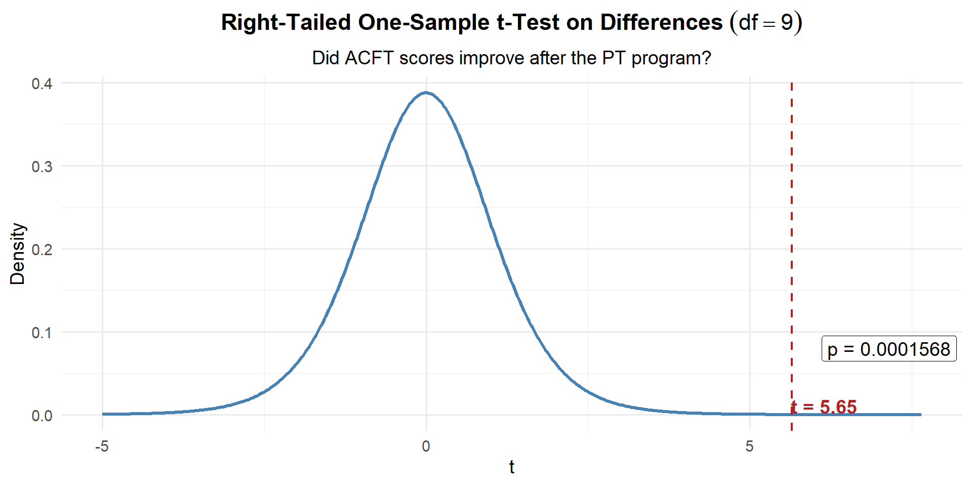
p_value <- 1 - pt(t_stat, df = n - 1)
p_value

[1] 0.0001569676

Step 5: Decide and Conclude

\(p < 0.001 \leq 0.05\). We reject \(H_0\). At the 5% significance level, there is strong evidence that the PT program improved ACFT scores. The average improvement was 12.1 points.

Confidence Interval for the Mean Difference

Just like any one-sample \(t\) CI:

\[\bar{d} \pm t_{\alpha/2, \, n-1} \cdot \frac{s_d}{\sqrt{n}}\]

t_crit <- qt(0.975, df = n - 1)
me <- t_crit * s_d / sqrt(n)
c(d_bar - me, d_bar + me)

[1]  7.254663 16.945337

We are 95% confident that the true average ACFT improvement is between 7.3 and 16.9 points.

Since the entire interval is above zero, this is consistent with rejecting \(H_0\).

Paired or Independent? How Do You Tell?

The Key Question

Ask yourself: Is there a natural one-to-one pairing between the observations?

Paired: Same person measured twice, left vs. right, before vs. after, matched subjects
Independent: Two separate groups with no connection between individual observations

Scenario	Design
50 Soldiers’ ACFT scores before and after a PT program	Paired
30 cadets from Co A vs. 35 cadets from Co B on a math exam	Independent
20 rifles tested with old method, then same 20 with new method	Paired
Reaction times of 25 caffeine users vs. 25 non-users	Independent
Each of 25 cadets rates difficulty of two courses	Paired

The Updated Inference Toolkit

Summary of Two-Sample Hypothesis Tests

	Two-Sample \(z\) (Large)	Two-Sample \(t\) (Small)	Paired \(t\)
Parameter	\(\mu_1 - \mu_2\)	\(\mu_1 - \mu_2\)	\(\mu_d\)
\(H_0\)	\(\mu_1 - \mu_2 = 0\)	\(\mu_1 - \mu_2 = 0\)	\(\mu_d = 0\)
Test Stat	\(z = \dfrac{\bar{x}_1 - \bar{x}_2}{SE}\)	\(t = \dfrac{\bar{x}_1 - \bar{x}_2}{SE}\)	\(t = \dfrac{\bar{d} - \Delta_0}{s_d / \sqrt{n}}\)
\(SE\)	\(\sqrt{s_1^2/n_1 + s_2^2/n_2}\)	\(\sqrt{s_1^2/n_1 + s_2^2/n_2}\)	\(s_d / \sqrt{n}\)
Distribution	\(N(0,1)\)	\(t_{df}\)	\(t_{n-1}\)
Conditions	\(n_1, n_2 \geq 30\)	Populations ~ Normal	Differences ~ Normal (or \(n \geq 30\))
Design	Independent groups	Independent groups	Same subjects measured twice

Decision rule is always the same: \(p \leq \alpha\) → Reject \(H_0\). \(p > \alpha\) → Fail to reject \(H_0\).

Board Problems

Problem 1: Body Armor Weight

Two companies test different body armor configurations. The S4 wants to know if there’s a difference in average load weight.

	Config A	Config B
\(n\)	10	12
\(\bar{x}\) (lbs)	34.2	31.8
\(s\)	3.5	4.1

Questions

Is this paired or independent? Why?
State the hypotheses for a two-tailed test.
Compute the test statistic, degrees of freedom, and \(p\)-value.
At \(\alpha = 0.05\), state your conclusion in context.

Answers

Independent. Different Soldiers in each group — no natural pairing.
\(H_0: \mu_A - \mu_B = 0\) vs. \(H_a: \mu_A - \mu_B \neq 0\)

n1 <- 10; n2 <- 12
xbar1 <- 34.2; xbar2 <- 31.8
s1 <- 3.5; s2 <- 4.1

se <- sqrt(s1^2 / n1 + s2^2 / n2)
t_stat <- (xbar1 - xbar2) / se
df <- (s1^2/n1 + s2^2/n2)^2 / ((s1^2/n1)^2/(n1-1) + (s2^2/n2)^2/(n2-1))
p_value <- 2 * (1 - pt(abs(t_stat), df = df))
t_stat

[1] 1.481077

df

[1] 19.97797

p_value

[1] 0.1541863

\[df = \frac{\left(\dfrac{3.5^2}{10} + \dfrac{4.1^2}{12}\right)^2}{\dfrac{\left(3.5^2/10\right)^2}{9} + \dfrac{\left(4.1^2/12\right)^2}{11}} = \frac{\left(1.225 + 1.401\right)^2}{\dfrac{1.225^2}{9} + \dfrac{1.401^2}{11}} = \frac{6.895}{0.167 + 0.178} = 19.98 \implies \lfloor df \rfloor = 19\]

\(p = 0.1542 > 0.05\), so we fail to reject \(H_0\). At the 5% significance level, there is not sufficient evidence of a difference in average load weight between the two configurations.

Problem 2: Land Navigation — Before and After Training

A platoon leader has 8 cadets complete a land navigation course, then puts them through a 2-week orienteering clinic and has them run the course again.

Cadet	1	2	3	4	5	6	7	8
Before (min)	52	48	61	55	44	58	50	63
After (min)	47	45	56	50	43	54	48	57

Questions

Why is this a paired design?
Compute the differences. What does a positive \(d_i\) (Before \(-\) After) mean?
State the hypotheses if we want to show the training reduced times.
Run the test and state your conclusion at \(\alpha = 0.05\).
Construct and interpret a 95% CI for \(\mu_d\).

Answers

The same 8 cadets are measured before and after. Each cadet is their own control.

before <- c(52, 48, 61, 55, 44, 58, 50, 63)
after  <- c(47, 45, 56, 50, 43, 54, 48, 57)
d <- before - after
d

[1] 5 3 5 5 1 4 2 6

Positive \(d_i\) means the cadet was faster after training (lower time).

\(H_0: \mu_d = 0\) vs. \(H_a: \mu_d > 0\) (training reduced times)

n <- length(d)
d_bar <- mean(d)
s_d <- sd(d)
t_stat <- d_bar / (s_d / sqrt(n))
t_stat

[1] 6.346766

p_value <- 1 - pt(t_stat, df = n - 1)
p_value

[1] 0.0001932116

\(p = 2e-04 \leq 0.05\), so we reject \(H_0\). At the 5% significance level, there is sufficient evidence that the orienteering clinic reduced land navigation times. The average improvement was 3.9 minutes.

t_crit <- qt(0.975, df = n - 1)
me <- t_crit * s_d / sqrt(n)
c(d_bar - me, d_bar + me)

[1] 2.431285 5.318715

We are 95% confident that the true average time reduction is between 2.43 and 5.32 minutes.

Problem 3: Paired or Independent?

For each scenario, state whether the data are paired or independent.

Questions

40 cadets from 1st Regiment vs. 45 cadets from 2nd Regiment compare ACFT scores.
30 patients have blood pressure measured before and 1 hour after taking a new medication.
A study compares test scores of 20 students who used a study app vs. 20 who did not.
Each of 15 Soldiers fires a qualification course with iron sights, then again with an optic.
First-born twins’ GPA compared to second-born twins’ GPA for 25 pairs.

Answers

Independent. Different cadets in each group.
Paired. Same patients before and after — each patient is their own control.
Independent. Different students in each group.
Paired. Same Soldiers fire under both conditions.
Paired. Each twin pair creates a natural match.

Problem 4: Screen Time Reduction

A wellness program claims to reduce cadets’ daily screen time. 20 cadets report average daily screen time (hours) before and after a 4-week program. Summary statistics for the differences (Before \(-\) After):

	\(n\)	\(\bar{d}\)	\(s_d\)
	20	0.8	1.5

Questions

State the hypotheses.
Compute the test statistic and \(p\)-value.
At \(\alpha = 0.05\), state your conclusion in context.
Construct a 95% CI for \(\mu_d\). Does it support the test result?

Answers

\(H_0: \mu_d = 0\) vs. \(H_a: \mu_d > 0\) (screen time decreased)

n <- 20; d_bar <- 0.8; s_d <- 1.5
t_stat <- d_bar / (s_d / sqrt(n))
t_stat

[1] 2.385139

p_value <- 1 - pt(t_stat, df = n - 1)
p_value

[1] 0.01382281

\(p = 0.0138 \leq 0.05\), so we reject \(H_0\). At the 5% significance level, there is sufficient evidence that the wellness program reduced daily screen time.

t_crit <- qt(0.975, df = n - 1)
me <- t_crit * s_d / sqrt(n)
c(d_bar - me, d_bar + me)

[1] 0.09797839 1.50202161

We are 95% confident that the true average screen time reduction is between 0.1 and 1.5 hours per day. The entire interval is above 0, consistent with rejecting \(H_0\).

Before You Leave

Today

Two-sample \(t\)-test: Same formula as the large-sample \(z\), but use the \(t\)-distribution when samples are small
Paired \(t\)-test: Compute differences \(d_i\), then it’s a one-sample \(t\)-test — nothing new!
Paired vs. Independent: Ask “are these the same subjects measured twice?”
Key difference: Independent → use \(SE = \sqrt{s_1^2/n_1 + s_2^2/n_2}\); Paired → compute differences first, then use \(SE = s_d/\sqrt{n}\)

Any questions?

Next Lesson

Lesson 24: Two Population Proportions

Check large-sample conditions for two proportions
Test \(p_1 - p_2\) using pooled SE
Construct and interpret a CI for \(p_1 - p_2\)

Upcoming Graded Events

WebAssign 9.2, 9.3 - Due before Lesson 24
WPR II - Lesson 27