Lesson 35: ANOVA I

The Project: Where You Should Be

The Project Peer Review due Lesson 36 – Come in to class with your 85% solution. Every person brings in 3 copies.

Project Links

Resource	Link
Project Instructions	Course Project Instructions (PDF)
Project Groups / Pairs	Project Pairs
Presentation Template	MA206X West Point Template (.pptx)
Army Vantage	Vantage Workspace

Example Write-Up: Sections 3.1 – 3.3

Below is the level of writing and analysis I expect on the project. The example uses simulated data for a fictional 2nd BCT, 10th Mountain Division (not your real brigade). Use it as a template for tone, structure, depth, and how to weave R output into narrative – not as content to copy.

3.1 Executive Summary

BLUF. 2nd BCT’s mean AFT score is statistically indistinguishable from the 360-point promotion standard, but roughly one in three Soldiers still scores below 360. Targeted remediation at the individual level – not brigade-wide PT – is the highest-leverage intervention.

Methods. We analyzed 592 individual Soldier records from Army Vantage (JAN – MAR 2026) after data cleaning. We ran a one-sample \(t\)-test against the 360 promotion standard, a two-sample \(t\)-test comparing Combat Arms vs. Combat Support AFT totals, and a multiple linear regression predicting AFT total score from time in service, body-fat percent, billet, and M4 score.

Key results.

Brigade mean AFT does not differ from the 360 standard at \(\alpha = 0.05\).
Combat Arms outscore Combat Support on the AFT by a meaningful margin (\(p < 0.001\)).
Body-fat percent and time in service are the strongest predictors of AFT performance.
Roughly 31% of Soldiers are below the 360 standard despite the brigade average clearing it.

Recommendation. Shift remediation resources from blanket unit PT to a body-composition-focused program for the below-360 cohort, prioritizing Combat Support companies.

3.2 Introduction

Problem statement. The brigade commander must decide how to allocate limited training time to maximize lethality. Brigade-level pass rates alone obscure who is at risk and why.

Objectives. (1) Determine whether mean brigade AFT performance meets the 360 promotion standard. (2) Identify subgroups with performance gaps. (3) Quantify which Soldier-level factors drive AFT performance.

Scope. 2nd BCT, 10th Mountain Division; data pulled from Army Vantage covering JAN – MAR 2026; starting roster of 612 Soldiers across 3 battalions.

Variable summary.

Variable	Type	Description
`aft_score_total`	Numeric (0–500)	Total AFT score (response of interest)
`billet`	Categorical	Combat Arms vs. Combat Support
`tis_years`	Numeric	Years on active duty
`age_bracket`	Categorical	18–25, 26–30, 31–35, 36+
`body_fat`	Numeric	Tape-test estimate (%)
`m4_score`	Numeric (0–40)	M4 qualification score

Data cleaning. We dropped records missing aft_score_total and records with body_fat outside [3%, 40%] (sensor/entry errors). No imputation was performed. Final analytic sample: \(n = 592\).

Descriptive statistics (key variables).

Variable	Mean (SD)
AFT total	392.1 (43.9)
TIS (yr)	6.1 (4.2)
Body fat (%)	19.3 (4.9)
M4 score	31.2 (3.9)

3.3 One-Sample Hypothesis Test

Question. Does 2nd BCT’s mean AFT score differ from the Army promotion standard of 360?

1. Exploratory Data Analysis.

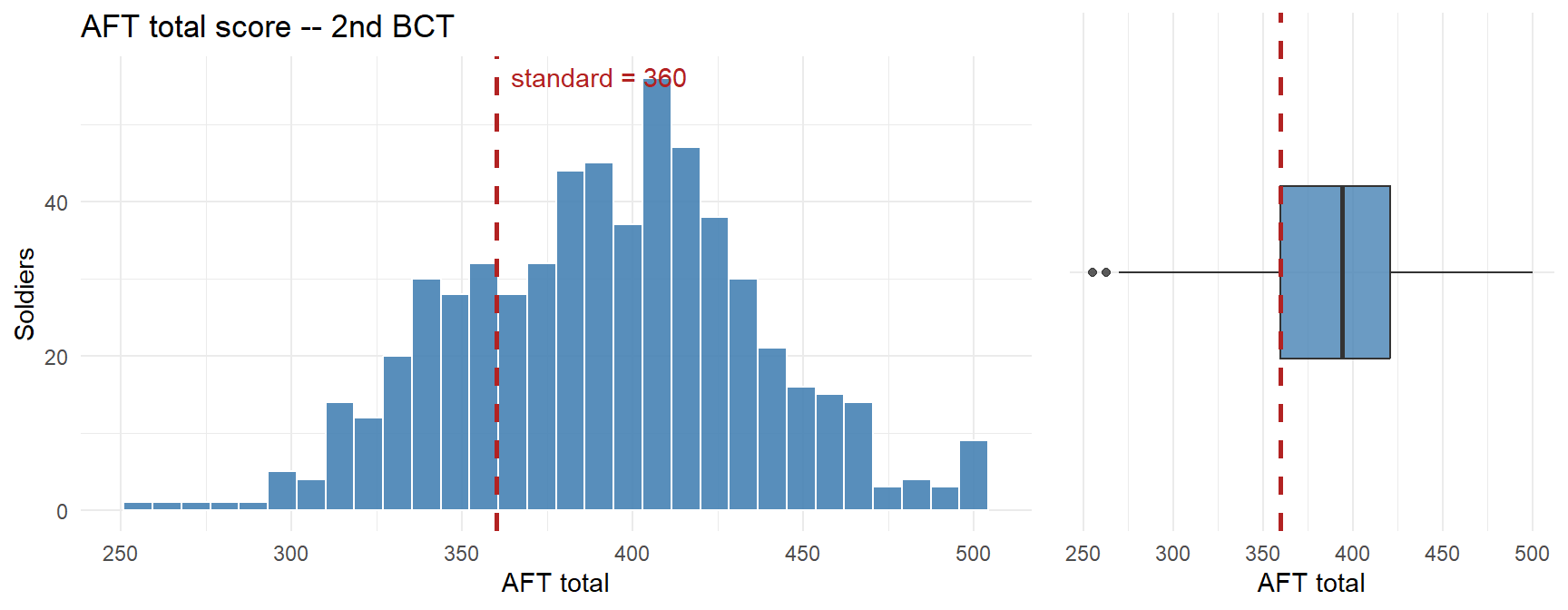
n	Mean	SD	Median	% below 360
592	392.1	43.9	394	24.0%

Observation: The distribution is roughly symmetric with a slight left tail. The brigade mean sits just above the standard, but nearly a third of the force is below it. The mean alone hides a substantial at-risk tail.

2. Methodology.

\(H_0:\ \mu = 360\)
\(H_a:\ \mu \ne 360\)
Procedure: one-sample \(t\)-test, two-sided.
Significance level: \(\alpha = 0.05\).
Assumptions:
- Independence: Soldiers are distinct records; reasonable.
- Normality: \(n = 592 \gg 30\), so CLT covers any mild non-normality seen in the EDA.
- Representative sample: Data are the full brigade roster for the window; we treat them as a sample of the brigade’s underlying performance process.

3. Results.


    One Sample t-test

data:  bde_clean$aft_score_total
t = 17.758, df = 591, p-value < 0.00000000000000022
alternative hypothesis: true mean is not equal to 360
95 percent confidence interval:
 388.5150 395.6066
sample estimates:
mean of x 
 392.0608

Test statistic: \(t = 17.76\) on \(591\) df.
p-value: \(0\).
95% CI for \(\mu\): \([388.5,\ 395.6]\).
Effect size: Cohen’s \(d = 0.73\) – negligible.
Decision: \(p = 0 < 0.05\), so we reject \(H_0\).

Interpretation. We do not have evidence that the brigade’s mean AFT score differs from the 360 promotion standard. Operationally, this is a mixed result: on average, 2nd BCT meets the standard, but the confidence interval straddles 360 and about a third of individual Soldiers still fail to clear it. Relying on the brigade mean would mask a real readiness problem at the Soldier level – the mean is a summary, not a roster. The one-sample test answers “is the average Soldier at standard?” but the commander’s real question is “how many Soldiers are not?” – which the two-sample and regression analyses in §3.4 and §3.5 address.

What We Did: Lessons 28, 30, 31, 32, 33

Lesson 28: Simple Linear Regression I

Least squares fits \(\hat{y} = b_0 + b_1 x\) by minimizing \(\sum(y_i - \hat{y}_i)^2\)
\(R^2\) = fraction of variability in \(y\) explained
Decompose variability: SST = SSR + SSE

Lesson 30: Simple Linear Regression II

Test the slope with \(t = b_1 / SE(b_1)\)
Prediction vs. mean-response intervals
Residual and QQ plots to assess adequacy

Lesson 31: Multiple Linear Regression I

Interpret each slope holding other variables constant
LINE assumptions: Linearity, Independence, Normality, Equal variance
Adjusted \(R^2\) and multicollinearity

Lesson 32: Multiple Linear Regression II

Categorical predictors via indicator variables with a reference level
Identify and control for confounders

Lesson 33: Multiple Linear Regression III

Interaction terms: effect of one predictor depends on another
Distinguish main effects from interaction effects

What We’re Doing: Lesson 35

Objectives

State ANOVA assumptions and hypotheses
Compute the \(F\)-statistic from sums of squares
Conduct one-way ANOVA tests
Report differences with CIs and effect sizes

Required Reading

Devore, Section 10.1

Break!

The Kids

In Memoriam: CPT Tim Cunningham

A moment to remember CPT Tim Cunningham.

Listen / read: Soldiers Try to Cope with Battlefield Losses – NPR (2008)

The Takeaway for Today

One-Way ANOVA Key Ideas

Goal: compare means across \(k \ge 3\) groups
Hypotheses:
- \(H_0: \mu_1 = \mu_2 = \cdots = \mu_k\)
- \(H_a:\) at least one \(\mu_i\) differs
Test statistic: \(F = \dfrac{MSR}{MSE}\)
Reject \(H_0\) when \(F\) is large (variation between groups exceeds variation within groups)

Motivating ANOVA: What If We Want a Lot of Pairwise Comparisons?

Start Simple: Two Companies

Suppose for your project you want to compare AFT scores (max 500) between two companies in a battalion – say A Co and B Co. Easy: two-sample t-test, done. One test, one p-value, one \(\alpha\).

head(A)

[1] 307.5771 334.6212 369.6961 301.7406 327.9937 333.3105

head(B)

[1] 298.7073 371.9309 345.0860 379.8051 367.2409 378.4735

First, look at the data:

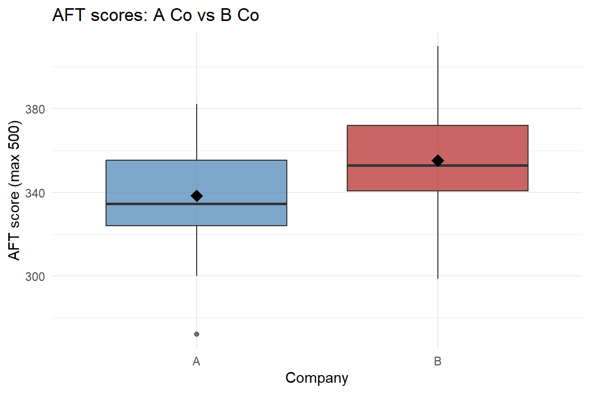
B Co sits a bit higher than A Co. Is the gap big enough to be real? Run the test:

t.test(A, B, alternative = "two.sided", mu = 0, conf.level = .95, paired = FALSE)


    Welch Two Sample t-test

data:  A and B
t = -2.1372, df = 47.799, p-value = 0.03773
alternative hypothesis: true difference in means is not equal to 0
95 percent confidence interval:
 -32.5258433  -0.9905815
sample estimates:
mean of x mean of y 
 338.3493  355.1076

The p-value is below \(0.05\), so we reject \(H_0\) – A Co and B Co really do differ. Clean result.

Now Add More Companies

But a battalion has A, B, C, and HHC. We want to know: “do any companies differ in average AFT score?”

How many pairwise comparisons is that?

\[ \binom{4}{2} = \frac{4 \cdot 3}{2} = 6 \text{ tests} \]

A vs B, A vs C, A vs HHC, B vs C, B vs HHC, C vs HHC.

Look at all four:

# A tibble: 8 × 2
# Groups:   company [4]
  score company
  <dbl> <fct>  
1  375. A      
2  308. A      
3  341. B      
4  372. B      
5  336. C      
6  354. C      
7  358. HHC    
8  338. HHC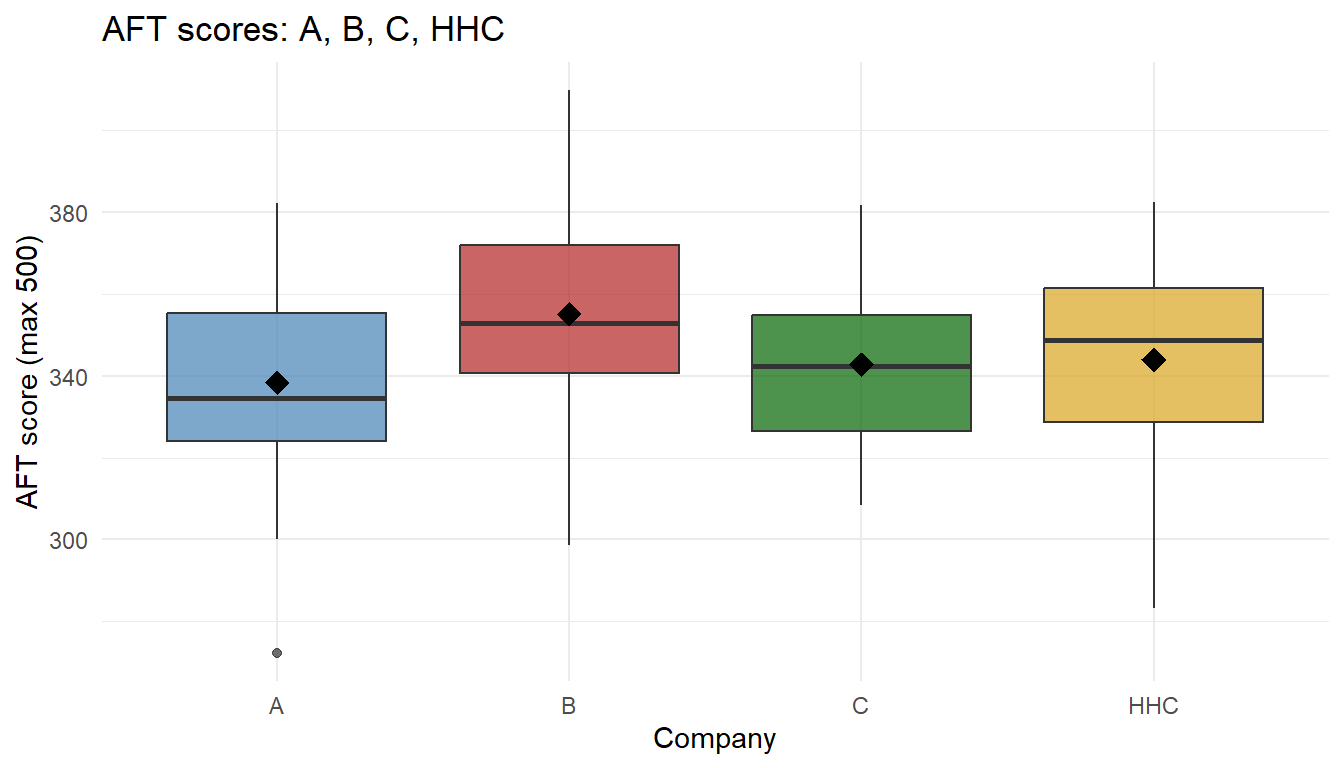

Some companies look different, others look similar – but our eyes are unreliable with this much overlap. Let’s run all six pairwise t-tests:

Comparison	Mean 1	Mean 2	Difference	p-value	Decision
A vs B	338.3	355.1	-16.8	0.0377	Reject H0 (significant)
A vs C	338.3	342.8	-4.4	0.5246	Fail to reject
A vs HHC	338.3	344.0	-5.7	0.4503	Fail to reject
B vs C	355.1	342.8	12.3	0.0690	Fail to reject
B vs HHC	355.1	344.0	11.1	0.1293	Fail to reject
C vs HHC	342.8	344.0	-1.2	0.8407	Fail to reject

Some pairs come back significant, others don’t. Each individual test was run at \(\alpha = 0.05\) – but we just ran six of them.

What Is \(\alpha\), Really?

When we run one test at \(\alpha = 0.05\), we’re saying:

“If \(H_0\) is true, I’m willing to accept a 5% chance of a false positive – concluding the means differ when they really don’t.”

That’s fine for one test. But we just ran six.

The Problem: False Positives Pile Up

If all 6 null hypotheses are true, and each test independently has a 5% chance of a false positive, the probability of at least one false positive across the family is:

\[ P(\text{at least one false positive}) = 1 - (1 - \alpha)^m = 1 - 0.95^6 \approx 0.265 \]

So with 4 companies and 6 pairwise tests at \(\alpha = 0.05\), there’s roughly a 26.5% chance we’ll claim somewhere that two companies differ – even if they are all identical.

This Is the Multiple Comparisons Problem

Run enough tests and you will find “significance” by pure chance. Your stated \(\alpha\) per test is not your real \(\alpha\) for the whole question.

How Do We Fix It?

One simple fix: use a stricter threshold on each test. If we want the family-wise false-positive rate to stay at 5%, we shrink each test’s \(\alpha\). The Bonferroni correction divides by the number of tests:

\[ \alpha^* = \frac{\alpha}{m} = \frac{0.05}{6} \approx 0.0083 \]

Now each pairwise test must clear a much smaller p-value to be called significant. Let’s redo the table with the corrected threshold:

Comparison	Mean 1	Mean 2	Difference	p-value	Decision (α* = 0.0083)
A vs B	338.3	355.1	-16.8	0.0377	Fail to reject
A vs C	338.3	342.8	-4.4	0.5246	Fail to reject
A vs HHC	338.3	344.0	-5.7	0.4503	Fail to reject
B vs C	355.1	342.8	12.3	0.0690	Fail to reject
B vs HHC	355.1	344.0	11.1	0.1293	Fail to reject
C vs HHC	342.8	344.0	-1.2	0.8407	Fail to reject

Now nothing is significant. Bonferroni controls the family-wise error rate, but the cost is obvious: it is very conservative – we may miss real differences that a single pre-planned t-test would have caught.

A Different Approach: One Big Question

Instead of running many small tests and patching up the error rate, we can ask one big question with a single test at level \(\alpha\):

“Are any of the group means different?”

That single test is ANOVA.

Building Intuition: What Does “Different Means” Look Like?

Before any math, let’s just look at group data. Here are four companies (A, B, C, HHC) and their AFT scores. In all four panels the group means are identical – it’s the within-group spread that changes.

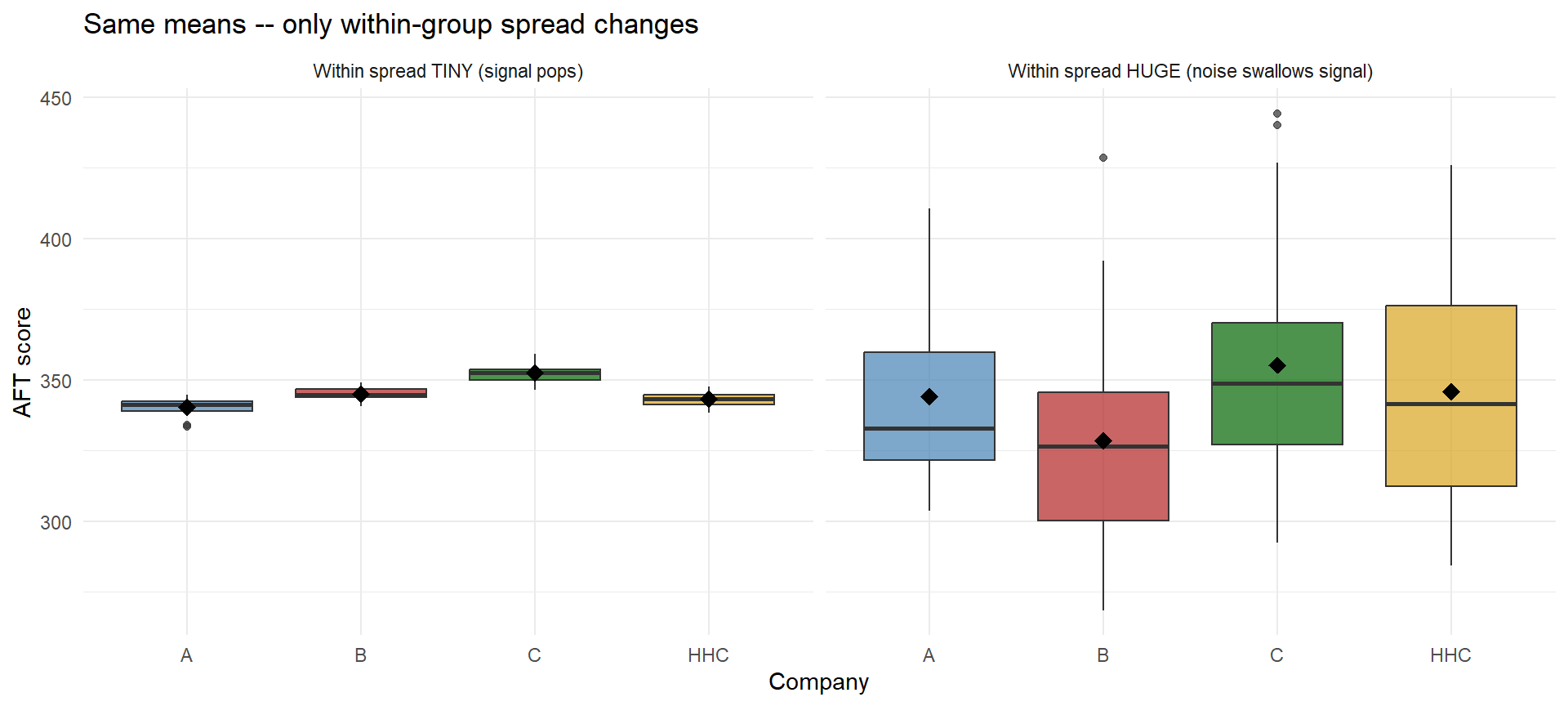
Same means, wildly different conclusions. When within-group spread is tiny (left), even a small gap between group means looks meaningful. When within-group spread is huge (right), the same gap vanishes into noise.

Now flip it: keep the within-group spread fixed and move the means around.

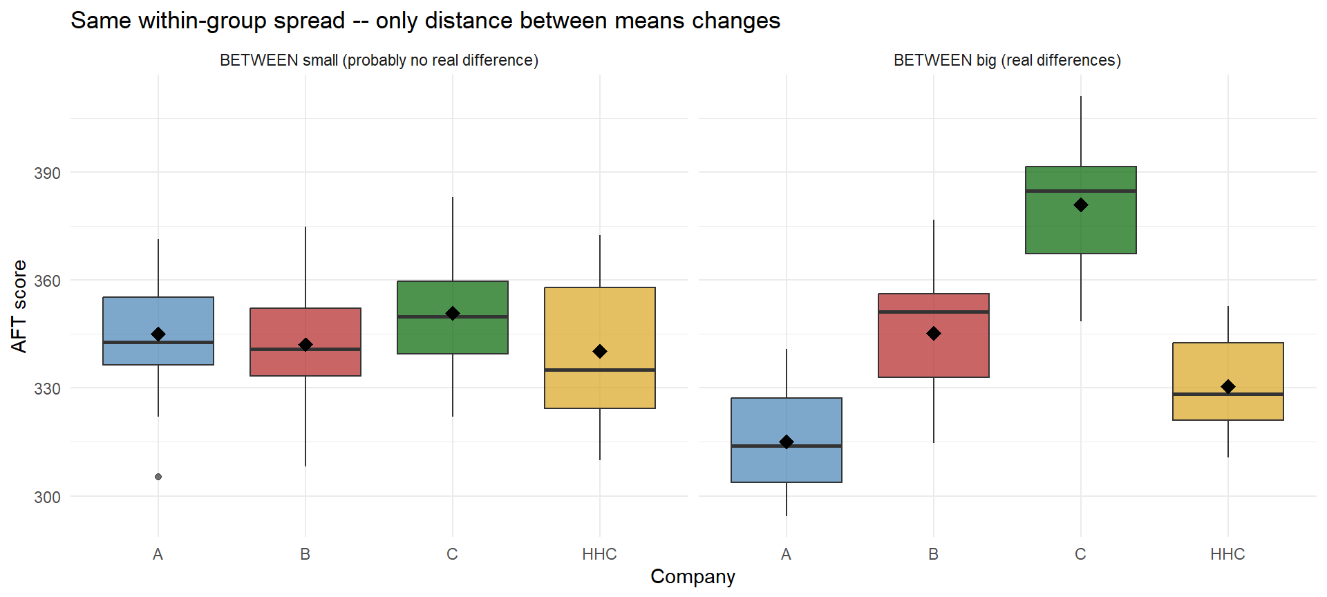
The punchline: whether the groups really differ depends on both how far apart the group means are and how noisy each group is. Next we need a way to quantify both.

Building ANOVA from the AFT Data

Here’s the boxplot we had from the motivation – the four companies’ AFT scores:

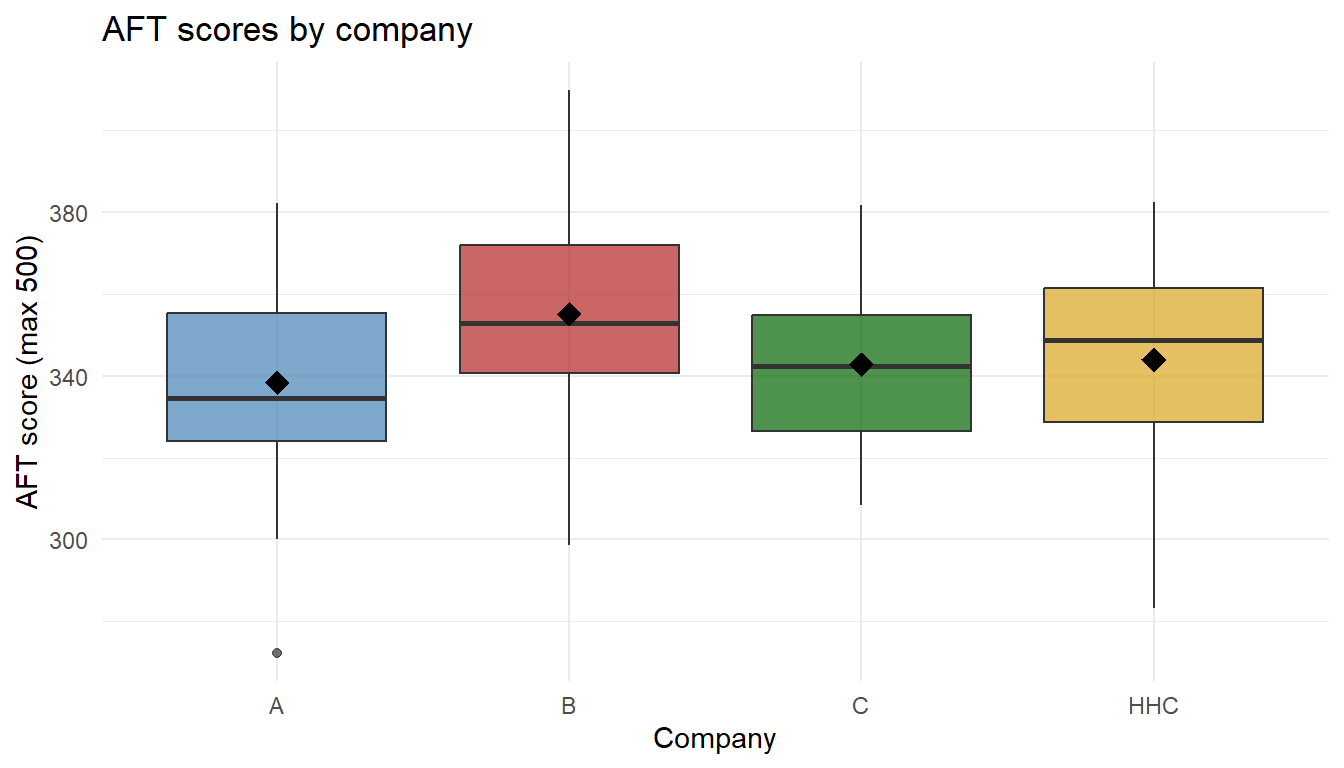
We need a way to mathematically codify this concept – specifically, to measure the two sources of variability at work here:

A measure of between-group variability – how spread out the group means are
A measure of within-group variability – how noisy each group is internally

Once we have both, we’ll combine them into a single ratio. Let’s build each one from scratch.

A bit of notation we’ll use:

\(k\) = number of groups; \(n_i\) = sample size in group \(i\); \(N = \sum n_i\) = total
\(\bar{x}_i\) = sample mean of group \(i\); \(\bar{x}\) = grand mean (mean of all data)

For our AFT data:

\[ k = 4, \qquad N = 100, \qquad \bar{x} = 345.07 \]

\[ \bar{x}_A = 338.35, \quad \bar{x}_B = 355.11, \quad \bar{x}_C = 342.78, \quad \bar{x}_{HHC} = 344.02 \]

Measuring Between-Group Variability

We want a number that’s big when the group means are spread out and small when they’re all close to the grand mean. The sum of squares between (a.k.a. sum of squares treatment) does that:

\[ SSR = \sum_{i=1}^{k} n_i \,(\bar{x}_i - \bar{x})^2 \]

And the mean square between just divides by its degrees of freedom:

\[ MSR = \frac{SSR}{k - 1} \]

SSR <- sum(group_n * (group_means - grand_mean)^2)
MSR <- SSR / (k - 1)

Plugging in:

\[ SSR = 25(338.35 - 345.07)^2 + 25(355.11 - 345.07)^2 + 25(342.78 - 345.07)^2 + 25(344.02 - 345.07)^2 = 3806.41 \]

\[ MSR = \frac{SSR}{k-1} = \frac{3806.41}{3} = 1268.8 \]

Measuring Within-Group Variability

Now a number for how noisy each group is. The sum of squares error sums every observation’s squared distance from its own group mean:

\[ SSE = \sum_{i=1}^{k} \sum_{j=1}^{n_i} (x_{ij} - \bar{x}_i)^2 \]

And the mean square error divides by its degrees of freedom:

\[ MSE = \frac{SSE}{N - k} \]

SSE <- sum((scores$score - group_means[scores$company])^2)
MSE <- SSE / (N - k)

\[ SSE = 5.955859\times 10^{4} \qquad\qquad MSE = \frac{5.955859\times 10^{4}}{96} = 620.4 \]

The Ratio

Combine them into a single signal-to-noise number:

\[ F = \frac{MSR}{MSE} = \frac{\text{between-group variability}}{\text{within-group variability}} \]

F_stat <- MSR / MSE

\[ F = \frac{1268.8}{620.4} = 2.045 \]

Stop and Think

What does this ratio tell us?

If the ratio is near 1, the between-group spread is about the same as the within-group noise. The gaps between company means look like ordinary random variation – consistent with all groups being the same.
If the ratio is much bigger than 1, the between-group spread is larger than ordinary noise can produce. That’s evidence the means are actually different.

So our decision depends on where our \(F\) value falls on a sliding scale: small → same, big → different.

Wait… this sounds like a hypothesis test.

It does, because it is. We can write the question formally:

\(H_0\): \(\mu_A = \mu_B = \mu_C = \mu_{HHC}\) (all company means are the same)
\(H_a\): at least one mean differs
Test statistic: \(F = MSR / MSE\), small under \(H_0\) and large under \(H_a\)

The only thing left: how big does \(F\) have to be before we call it “big”?

How Big Is Big Enough? The F Distribution

Under \(H_0\) (all group means equal), the ratio \(F = MSR/MSE\) follows an F distribution with \(k-1\) numerator df (between) and \(N-k\) denominator df (within):

\[ F \;\sim\; F_{\,k-1,\; N-k} \qquad\text{when } H_0 \text{ is true} \]

For our AFT data: \(k - 1 = 3\) and \(N - k = 96\). Plot the null distribution and mark our observed \(F\):

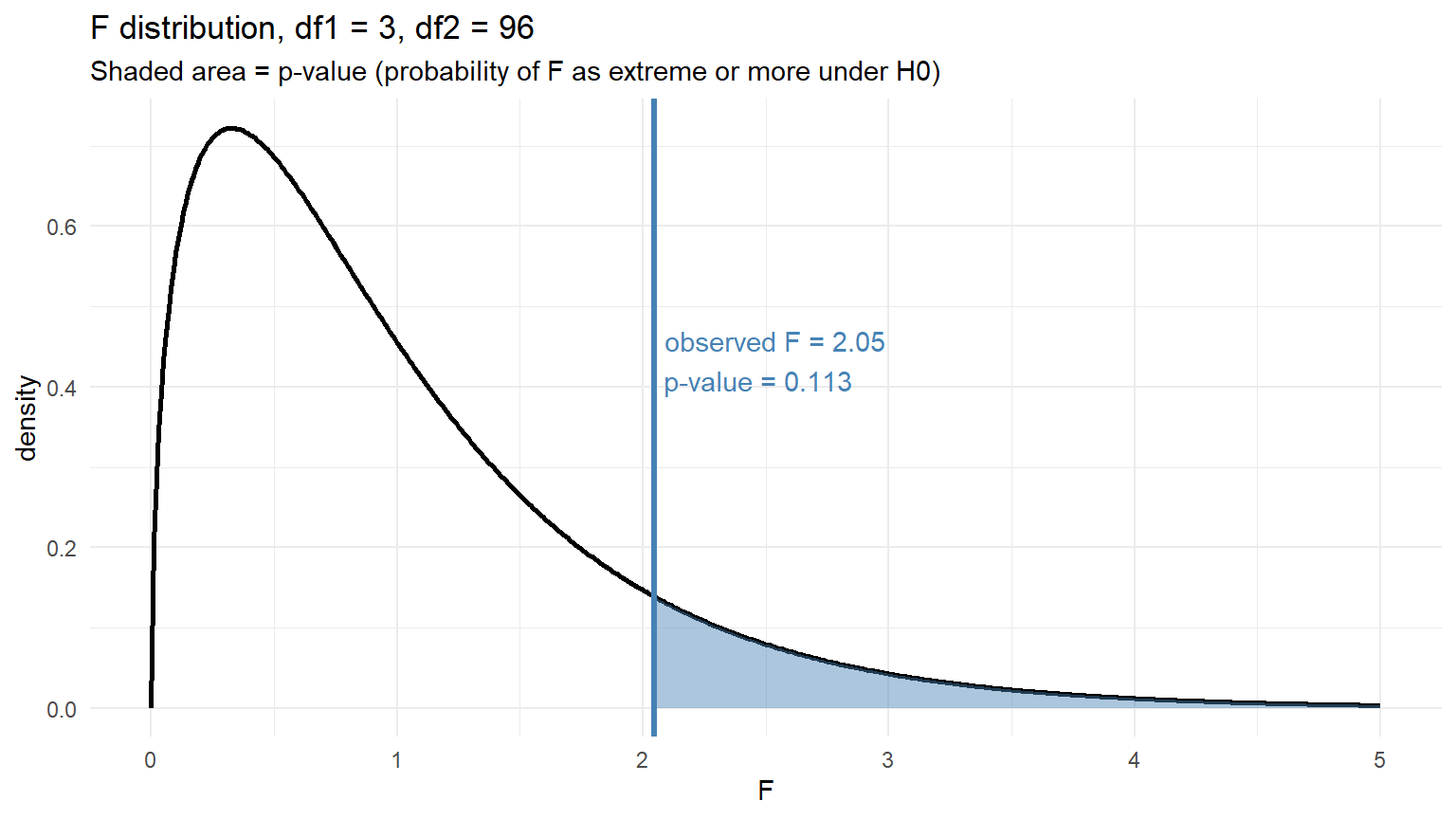
Blue line = our observed \(F\)
Blue shaded area = the p-value – the probability under \(H_0\) of getting an \(F\) at least as extreme as ours

Our Conclusion on the AFT Data

If the shaded area (the p-value) is smaller than \(\alpha = 0.05\), we reject \(H_0\) and conclude that at least one company mean differs from the others. If not, we fail to reject – the data don’t give us enough evidence to say any company mean is different.

ANOVA tells us that a difference exists, not which pair. Multiple-comparison procedures (Tukey HSD, Lesson 38) pick up from there.

Doing This in R with `aov()`

You don’t have to compute any of this by hand. R’s aov() builds the whole ANOVA table from a formula outcome ~ group.

Step 1: fit the model. The formula reads “score as a function of company,” and data = scores tells R which dataframe to pull the columns from.

fit_aov <- aov(score ~ company, data = scores)

Step 2: look at the ANOVA table with summary():

summary(fit_aov)

            Df Sum Sq Mean Sq F value Pr(>F)
company      3   3806  1268.8   2.045  0.113
Residuals   96  59559   620.4

Match the output to what we just did by hand:

`aov()` column	What it is	Our hand value
`Df`	degrees of freedom	\(k-1 = 3\) and \(N-k = 96\)
`Sum Sq`	sum of squares	\(SSR\) and \(SSE\)
`Mean Sq`	mean squares	\(MSR\) and \(MSE\)
`F value`	the F-statistic	\(MSR / MSE\)
`Pr(>F)`	the p-value	shaded area on our F plot

If you want just the p-value for a calculation, pull it out directly:

anova_summary <- summary(fit_aov)
anova_summary[[1]]$`Pr(>F)`[1]

[1] 0.1126863

Assumptions (check these before trusting the F-test)

ANOVA Assumptions

Independent observations within and between groups
Normality within each group (or large \(n_i\) so the CLT kicks in)
Equal variances across groups (rule of thumb: largest SD \(\le 2 \times\) smallest SD)

The ANOVA Intuition (take this with you)

Whether group means “really differ” depends on two things:

How far apart the group means are (between-group variability)
How noisy the data are within each group (within-group variability)

The F-statistic is literally the ratio of these two things:

\[ F = \frac{\text{between-group variability}}{\text{within-group variability}} = \frac{MSR}{MSE} \]

Big between, small within → \(F\) large → evidence the groups differ
Small between, big within → \(F\) near 1 → evidence consistent with equal means

It’s a signal-to-noise ratio.

Another Example: Five MOS Branches

Same idea, new data. Suppose we pull 2-mile run times (minutes) from Soldiers across five MOS branches – Combat Engineer (12B), Armor (19K), Artillery (13B), Signal (25U), and Infantry (11B) – and want to know if any branch differs on average.

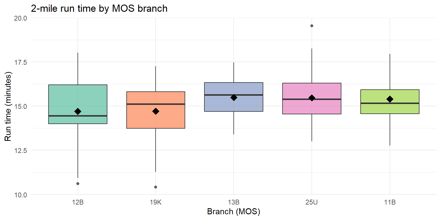
12B looks fastest, 11B slowest, with the other three branches in between. Does ANOVA agree that the gap is real?

Hypotheses:

\(H_0:\ \mu_{12B} = \mu_{19K} = \mu_{13B} = \mu_{25U} = \mu_{11B}\)
\(H_a:\) at least one branch mean differs

Fit the model:

mos_fit <- aov(run_time ~ branch, data = mos_data)
summary(mos_fit)

             Df Sum Sq Mean Sq F value Pr(>F)  
branch        4   20.1   5.020   2.201 0.0718 .
Residuals   145  330.8   2.281                 
---
Signif. codes:  0 '***' 0.001 '**' 0.01 '*' 0.05 '.' 0.1 ' ' 1

Read the table. With \(k = 5\) branches and \(N = 150\) Soldiers, df = (4, 145). The \(F\)-statistic is large and the p-value is far below \(0.05\), so we reject \(H_0\): mean 2-mile run time differs across branches.

Plot the F-statistic against the null distribution:

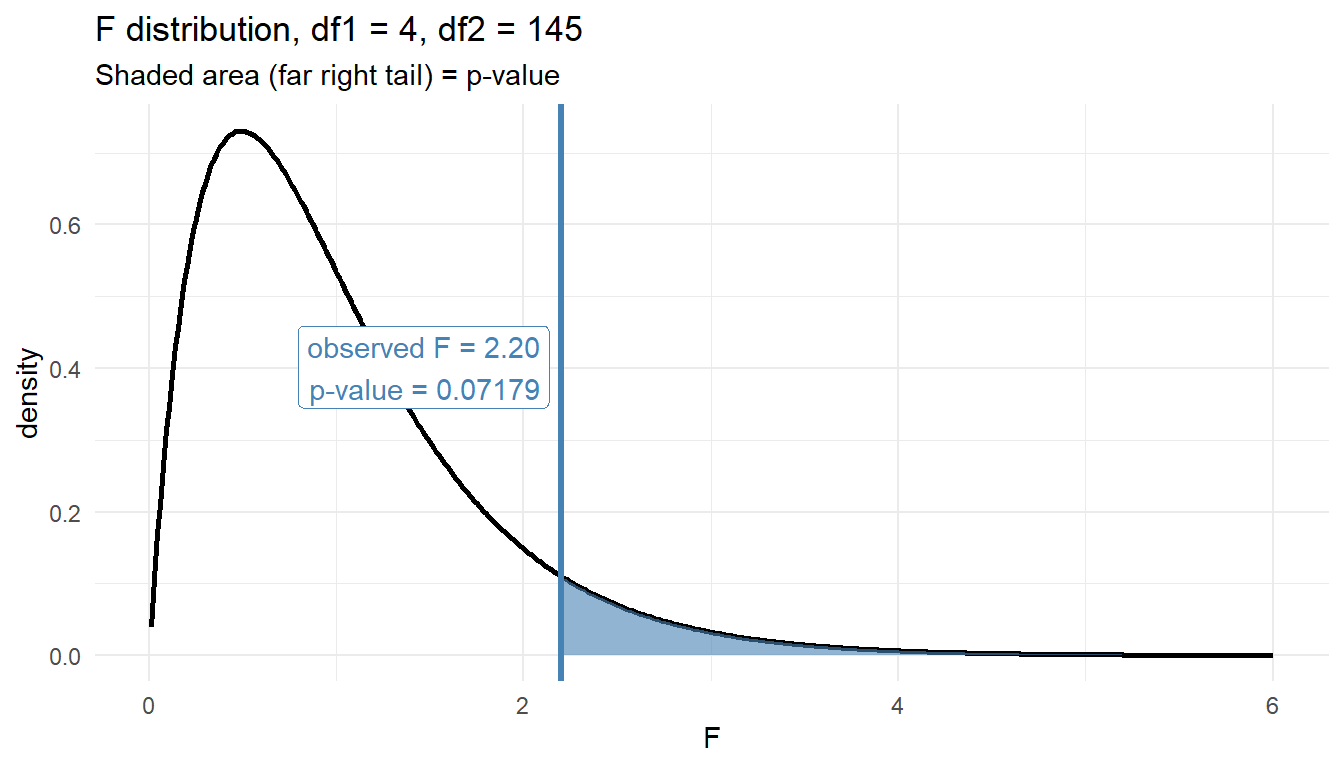
Our observed \(F\) sits far into the right tail of \(F_{4,145}\) – essentially no area remains beyond it, which is why the p-value is so small.

ANOVA does not tell us which pairs differ – the boxplot suggests 12B leads and 11B trails, but confirming specific pairwise gaps is a job for Tukey HSD in Lesson 38.

Board Problems

Problem 1: State the Hypotheses

A battalion S-3 wants to know if average time-to-qualify on the M4 differs across three companies (Alpha, Bravo, Charlie).

Questions

Write \(H_0\) and \(H_a\).
What are the degrees of freedom for the \(F\)-statistic if 15 soldiers are sampled from each company?

Answers

\(H_0: \mu_A = \mu_B = \mu_C\) vs. \(H_a:\) at least one company mean differs.
\(k = 3\), \(N = 45\), so df = (2, 42): between \(= k - 1 = 2\), within \(= N - k = 42\).

Problem 2: Compute the F-Statistic

You’re given the following ANOVA table with missing values:

Source	df	SS	MS	F
Branch	2	24.0	?	?
Error	27	54.0	?
Total	29	78.0

Questions

Compute \(MSR\), \(MSE\), and \(F\).
What is \(\eta^2\)?

Answers

\(MSR = 24/2 = \mathbf{12}\), \(MSE = 54/27 = \mathbf{2}\), \(F = 12/2 = \mathbf{6}\).
\(\eta^2 = 24/78 \approx \mathbf{0.308}\) – a large effect. Branch explains about 31% of the variability in the outcome.

Problem 3: Assumption Check

Group SDs for run times across four companies are: 0.9, 1.1, 1.2, and 2.8 minutes.

Question

Is the equal-variance assumption reasonable? What should you do?

Answer

No. Largest SD (\(2.8\)) is more than \(2\times\) smallest (\(0.9\)). Options:

Transform the outcome (log, square-root) and recheck
Investigate the outlier group – a big SD often means contamination or a different process

Problem 4: Interpret a Result

A company commander runs an ANOVA comparing marksmanship scores across three training methods. Output:

              Df  Sum Sq  Mean Sq  F value  Pr(>F)
method         2    180     90.0     7.5    0.002
Residuals     42    504     12.0
Total         44    684

Questions

State the conclusion at \(\alpha = 0.05\).
What is \(\eta^2\), and what does it mean?
What’s the next question the commander should ask?

Answers

\(p = 0.002 < 0.05\): reject \(H_0\). There is strong evidence that mean marksmanship scores differ across at least one pair of training methods.
\(\eta^2 = 180/684 \approx \mathbf{0.263}\) – training method explains about 26% of variability in scores. Large effect.
Which methods differ? ANOVA only flags that some pair differs. Pairwise comparisons (Tukey HSD) in Lesson 38 tell you which.

Before You Leave

Today

ANOVA compares \(\ge 3\) means with a single test at level \(\alpha\)
The \(F\)-statistic is the ratio of between-group to within-group variability
Always check assumptions and report an effect size with the \(p\)-value
ANOVA tells you that groups differ, not which pairs

Any questions?

Next Lesson

Lesson 36: ANOVA I (continued)

Continue one-way ANOVA
Tech Report due today

Upcoming Graded Events

Tech Report – Due Lesson 36
Project Presentation – Lessons 39–40
TEE – End of course

Lesson 35: ANOVA I

The Project: Where You Should Be

Example Write-Up: Sections 3.1 – 3.3

3.1 Executive Summary

3.2 Introduction

3.3 One-Sample Hypothesis Test

What We Did: Lessons 28, 30, 31, 32, 33

What We’re Doing: Lesson 35

Objectives

Required Reading

Break!

The Kids

In Memoriam: CPT Tim Cunningham

The Takeaway for Today

Motivating ANOVA: What If We Want a Lot of Pairwise Comparisons?

Start Simple: Two Companies

Now Add More Companies

What Is \(\alpha\), Really?

The Problem: False Positives Pile Up

How Do We Fix It?

A Different Approach: One Big Question

Building Intuition: What Does “Different Means” Look Like?

Building ANOVA from the AFT Data

Measuring Between-Group Variability

Measuring Within-Group Variability

The Ratio

Stop and Think

How Big Is Big Enough? The F Distribution

Our Conclusion on the AFT Data

Doing This in R with aov()

Assumptions (check these before trusting the F-test)

Another Example: Five MOS Branches

Board Problems

Problem 1: State the Hypotheses

Problem 2: Compute the F-Statistic

Problem 3: Assumption Check

Problem 4: Interpret a Result

Before You Leave

Today

Next Lesson

Upcoming Graded Events

Doing This in R with `aov()`