Lesson 13: Normal Distribution
The normal distribution shows up everywhere — heights, test scores, measurement errors. Today we learn how to work with it.
What We Did: Lessons 6–12
NoteReview: Lessons 6–12
NoteLesson 6: Probability Basics
Sample Spaces and Events:
- Sample space \(S\) = set of all possible outcomes
- Event = subset of the sample space
- Operations: Union (\(A \cup B\)), Intersection (\(A \cap B\)), Complement (\(A^c\))
Kolmogorov Axioms:
- \(P(A) \geq 0\)
- \(P(S) = 1\)
- For mutually exclusive events: \(P(A \cup B) = P(A) + P(B)\)
Key Rules:
- Complement Rule: \(P(A^c) = 1 - P(A)\)
- Addition Rule: \(P(A \cup B) = P(A) + P(B) - P(A \cap B)\)
NoteLesson 7: Conditional Probability
Conditional Probability: \[P(A \mid B) = \frac{P(A \cap B)}{P(B)}\]
Multiplication Rule: \[P(A \cap B) = P(A) \cdot P(B \mid A) = P(B) \cdot P(A \mid B)\]
Law of Total Probability: \[P(A) = P(B) \cdot P(A \mid B) + P(B^c) \cdot P(A \mid B^c)\]
Bayes’ Theorem: \[P(B \mid A) = \frac{P(B) \cdot P(A \mid B)}{P(B) \cdot P(A \mid B) + P(B^c) \cdot P(A \mid B^c)}\]
NoteLesson 8: Counting & Independence
Counting Formulas:
| With Replacement | Without Replacement | |
|---|---|---|
| Ordered | \(n^k\) | \(P(n,k) = \frac{n!}{(n-k)!}\) |
| Unordered | \(\binom{n+k-1}{k}\) | \(\binom{n}{k} = \frac{n!}{k!(n-k)!}\) |
Independence:
- \(A\) and \(B\) are independent if \(P(A \cap B) = P(A) \cdot P(B)\)
- Equivalently: \(P(A \mid B) = P(A)\)
- Independent \(\neq\) Mutually Exclusive!
NoteLesson 9: Discrete Random Variables
Random Variables:
- A random variable \(X\) assigns a numerical value to each outcome in a sample space
- Discrete RVs take finite or countably infinite values
PMF: \(p(x) = P(X = x)\) with \(p(x) \geq 0\) and \(\sum p(x) = 1\)
CDF: \(F(x) = P(X \leq x) = \sum_{y \leq x} p(y)\)
Expected Value: \(E(X) = \sum x \cdot p(x)\)
Variance: \(Var(X) = \sum (x - \mu)^2 \cdot p(x) = E(X^2) - [E(X)]^2\)
NoteLesson 10: Binomial Distribution
BINS Conditions:
- Binary outcomes (success/failure)
- Independent trials
- Number of trials is fixed (\(n\))
- Same probability (\(p\)) each trial
Key Formulas: If \(X \sim \text{Binomial}(n, p)\):
- PMF: \(P(X = x) = \binom{n}{x} p^x (1-p)^{n-x}\)
- Mean: \(E(X) = np\)
- Variance: \(Var(X) = np(1-p)\)
R Functions: dbinom(x, size, prob) for PMF, pbinom(x, size, prob) for CDF
NoteLesson 11: Poisson Distribution
When to Use Poisson:
- Counting events in a fixed interval (time, area, volume)
- Events occur independently at a constant average rate \(\lambda\)
Key Formulas: If \(X \sim \text{Poisson}(\lambda)\):
- PMF: \(P(X = x) = \frac{e^{-\lambda} \lambda^x}{x!}, \quad x = 0, 1, 2, \ldots\)
- Mean: \(E(X) = \lambda\)
- Variance: \(Var(X) = \lambda\)
R Functions: dpois(x, lambda) for PMF, ppois(x, lambda) for CDF
NoteLesson 12: Continuous Random Variables
Continuous vs. Discrete:
- Discrete RVs: probabilities come from a PMF — \(P(X = x)\)
- Continuous RVs: probabilities come from areas under a PDF — \(P(a \leq X \leq b) = \int_a^b f(x)\,dx\)
Probability Density Function (PDF): \(f(x)\) where:
- \(f(x) \geq 0\) for all \(x\)
- \(\int_{-\infty}^{\infty} f(x)\,dx = 1\)
- \(P(a \leq X \leq b) = \int_a^b f(x)\,dx\)
CDF: \(F(x) = P(X \leq x) = \int_{-\infty}^{x} f(t)\,dt\)
Key Facts:
- \(P(X = c) = 0\) for any single value \(c\)
- \(E(X) = \int x \cdot f(x)\,dx\)
- \(Var(X) = E(X^2) - [E(X)]^2\)
What We’re Doing: Lesson 13
Objectives
- Standardize and use normal probabilities
- Find normal quantiles for given tail areas
- Assess plausibility using normal models
Required Reading
Devore, Section 4.3
WPR I Overview
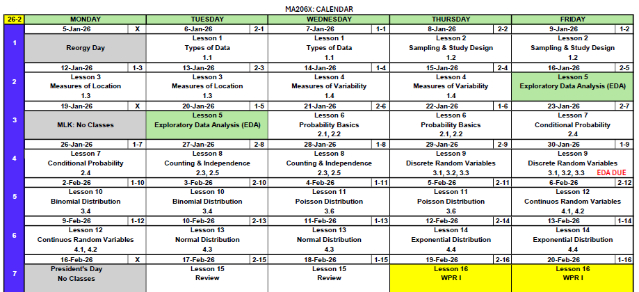
WPR I is Lesson 16 and covers all concepts from Lessons 6–14.
Study Materials (also available on Canvas)
No R on WPR I
There will be no R / no technology on WPR I. This means you need to know how to set up problems up to the point where you’d need technology to finish.
For example, if \(X \sim \text{Poisson}(\lambda = 3)\) and you need \(P(X \leq 2)\):
\[P(X \leq 2) = \sum_{x=0}^{2} \frac{e^{-\lambda}\lambda^x}{x!}\]
Or you can write: \(P(X \leq 2)\) = ppois(2, lambda = 3).
Break!
Reese
Cal
Army


The Takeaway for Today
NoteKey Concepts: Normal Distribution
The Normal Distribution: If \(X \sim N(\mu, \sigma^2)\):
- Bell-shaped, symmetric about \(\mu\)
- Defined by two parameters: mean \(\mu\) (center) and standard deviation \(\sigma\) (spread)
- \(f(x) = \frac{1}{\sigma\sqrt{2\pi}} e^{-\frac{(x-\mu)^2}{2\sigma^2}}\)
The Standard Normal: \(Z \sim N(0, 1)\)
Standardization: Convert any normal to standard normal: \[Z = \frac{X - \mu}{\sigma}\]
Unstandardization: Convert back: \[X = \mu + Z\sigma\]
R Functions:
pnorm(x, mean, sd)— CDF: \(P(X \leq x)\) (forward: value → probability)qnorm(p, mean, sd)— Quantile: find \(x\) such that \(P(X \leq x) = p\) (backward: probability → value)dnorm(x, mean, sd)— PDF: \(f(x)\) (density, not probability)
The Z Table:
- Gives \(\Phi(z) = P(Z \leq z)\) for \(Z \sim N(0,1)\)
- Forward: Standardize with \(z = \frac{x - \mu}{\sigma}\), look up \(z\) in table
- Backward (Quantile): Find probability \(p\) in the body of the table, read off \(z\), then \(x = \mu + z\sigma\)
Empirical Rule (68-95-99.7):
- 68% of data within \(\mu \pm \sigma\)
- 95% of data within \(\mu \pm 2\sigma\)
- 99.7% of data within \(\mu \pm 3\sigma\)
The Normal Distribution
Why the Normal?
The normal distribution is the most important distribution in statistics. It appears everywhere:
- Physical measurements (heights, weights, temperatures)
- Test scores (APFT, SAT, marksmanship)
- Measurement errors in equipment
- Sums and averages of many independent quantities (Central Limit Theorem — Lesson 17!)
The PDF
ImportantNormal Distribution
A continuous random variable \(X\) has a normal distribution with parameters \(\mu\) and \(\sigma\) (where \(\sigma > 0\)) if the PDF is:
\[f(x) = \frac{1}{\sigma\sqrt{2\pi}} e^{-\frac{(x-\mu)^2}{2\sigma^2}}, \quad -\infty < x < \infty\]
We write \(X \sim N(\mu, \sigma^2)\).
- \(\mu\) = mean (center of the bell curve)
- \(\sigma\) = standard deviation (controls the spread)
- \(\sigma^2\) = variance
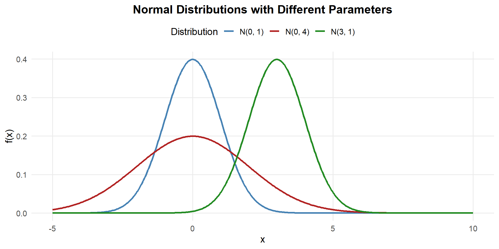
Key observations:
- Changing \(\mu\) shifts the curve left or right
- Changing \(\sigma\) stretches or compresses the curve
- The curve is always symmetric about \(\mu\)
- The total area under every normal curve is 1
Mean, Variance, and Standard Deviation
ImportantMean, Variance, and SD of the Normal Distribution
If \(X \sim N(\mu, \sigma^2)\) with PDF \(f(x) = \frac{1}{\sigma\sqrt{2\pi}} e^{-\frac{(x-\mu)^2}{2\sigma^2}}\), then:
\[E(X) = \mu\]
\[Var(X) = \sigma^2\]
\[SD(X) = \sigma\]
The parameters \(\mu\) and \(\sigma\) directly are the mean and standard deviation — that’s why we name them that way!
NoteDerivation: E(X) = μ (just FYI — not required)
Starting from the definition of expected value for a continuous RV:
\[E(X) = \int_{-\infty}^{\infty} x \cdot \frac{1}{\sigma\sqrt{2\pi}} e^{-\frac{(x-\mu)^2}{2\sigma^2}}\,dx\]
Substitute \(u = \frac{x - \mu}{\sigma}\), so \(x = \mu + \sigma u\) and \(dx = \sigma\,du\):
\[E(X) = \int_{-\infty}^{\infty} (\mu + \sigma u) \cdot \frac{1}{\sigma\sqrt{2\pi}} e^{-u^2/2} \cdot \sigma\,du\]
\[= \int_{-\infty}^{\infty} (\mu + \sigma u) \cdot \frac{1}{\sqrt{2\pi}} e^{-u^2/2}\,du\]
Split into two integrals:
\[= \mu \underbrace{\int_{-\infty}^{\infty} \frac{1}{\sqrt{2\pi}} e^{-u^2/2}\,du}_{= 1 \text{ (total area under std normal)}} + \sigma \underbrace{\int_{-\infty}^{\infty} u \cdot \frac{1}{\sqrt{2\pi}} e^{-u^2/2}\,du}_{= 0 \text{ (odd function, symmetric limits)}}\]
\[\boxed{E(X) = \mu}\]
NoteDerivation: Var(X) = σ² (just FYI — not required)
Using \(Var(X) = E(X^2) - [E(X)]^2\), we need \(E(X^2)\).
With the same substitution \(u = \frac{x - \mu}{\sigma}\):
\[E(X^2) = \int_{-\infty}^{\infty} (\mu + \sigma u)^2 \cdot \frac{1}{\sqrt{2\pi}} e^{-u^2/2}\,du\]
\[= \int_{-\infty}^{\infty} (\mu^2 + 2\mu\sigma u + \sigma^2 u^2) \cdot \frac{1}{\sqrt{2\pi}} e^{-u^2/2}\,du\]
Split into three integrals:
\[= \mu^2 \underbrace{\int \frac{1}{\sqrt{2\pi}} e^{-u^2/2}\,du}_{=1} + 2\mu\sigma \underbrace{\int u \cdot \frac{1}{\sqrt{2\pi}} e^{-u^2/2}\,du}_{=0} + \sigma^2 \underbrace{\int u^2 \cdot \frac{1}{\sqrt{2\pi}} e^{-u^2/2}\,du}_{=1 \text{ (integration by parts)}}\]
The last integral equals 1 (this is \(E(Z^2)\) where \(Z \sim N(0,1)\), and since \(E(Z) = 0\), we have \(E(Z^2) = Var(Z) + [E(Z)]^2 = 1 + 0 = 1\)).
\[E(X^2) = \mu^2 + \sigma^2\]
Therefore:
\[Var(X) = E(X^2) - [E(X)]^2 = (\mu^2 + \sigma^2) - \mu^2\]
\[\boxed{Var(X) = \sigma^2}\]
Computing Normal Probabilities
R Functions for the Normal Distribution
ImportantR Functions
pnorm(x, mean, sd)— CDF: \(P(X \leq x)\)qnorm(p, mean, sd)— Quantile: find \(x\) such that \(P(X \leq x) = p\)dnorm(x, mean, sd)— PDF: \(f(x)\)dnormto compute probabilities.
Suppose the maximum deadlift weight (in lbs) for male cadets follows a normal distribution with \(\mu = 340\) and \(\sigma = 40\).
\(P(X < a)\) — Less Than
What proportion of cadets deadlift less than 300 lbs?
Formally, this is an integral:
\[P(X < 300) = \int_{-\infty}^{300} \frac{1}{40\sqrt{2\pi}} e^{-\frac{(x-340)^2}{2(40)^2}}\,dx\]
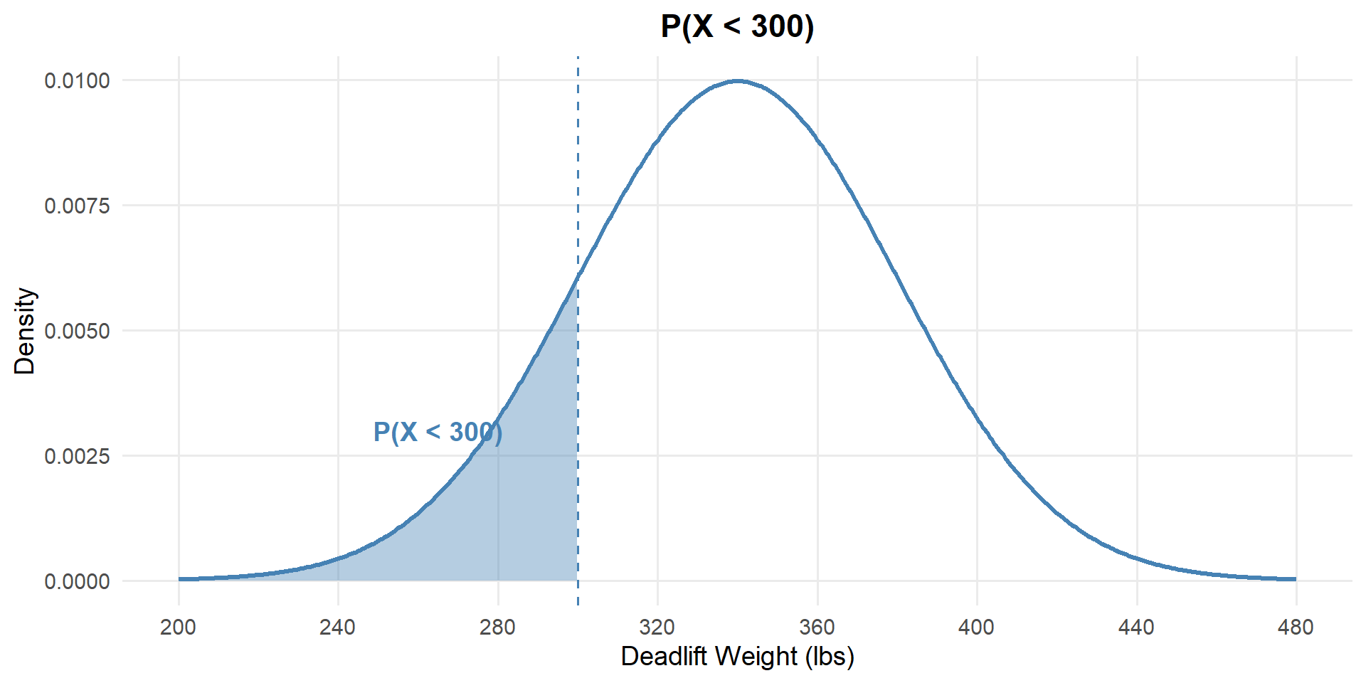
That integral is not fun to compute by hand — and we never will! Instead, pnorm does it for us:
# P(X < 300)
pnorm(300, mean = 340, sd = 40)
[1] 0.1586553About 15.9% of cadets deadlift less than 300 lbs.
\(P(X > a)\) — Greater Than
What proportion of cadets deadlift more than 400 lbs?
\[P(X > 400) = \int_{400}^{\infty} \frac{1}{40\sqrt{2\pi}} e^{-\frac{(x-340)^2}{2(40)^2}}\,dx\]
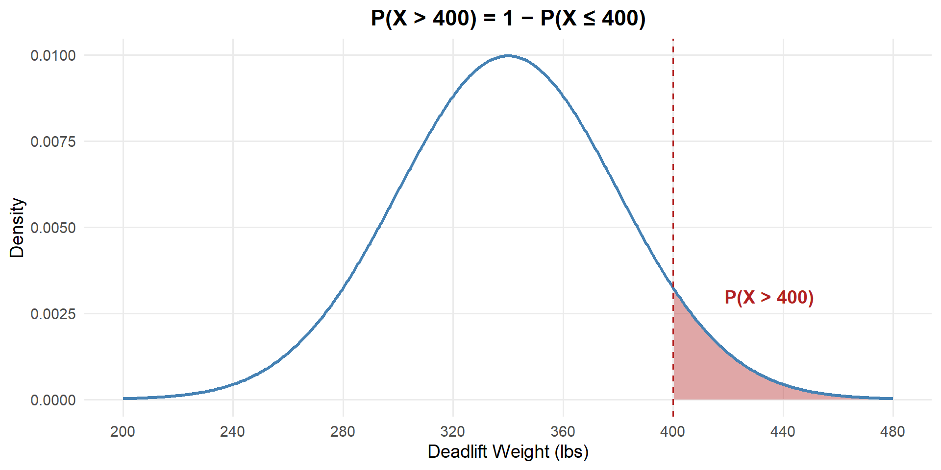
Again, we won’t touch that integral. Since pnorm gives \(P(X \leq x)\), we subtract from 1 to get the upper tail:
# P(X > 400) = 1 - P(X <= 400)
1 - pnorm(400, mean = 340, sd = 40)
[1] 0.0668072About 6.7% of cadets deadlift more than 400 lbs.
\(P(a < X < b)\) — Between Two Values
What proportion of cadets deadlift between 300 and 380 lbs?
\[P(300 < X < 380) = \int_{300}^{380} \frac{1}{40\sqrt{2\pi}} e^{-\frac{(x-340)^2}{2(40)^2}}\,dx\]
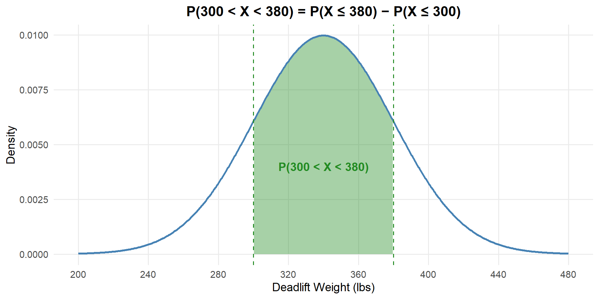
Same idea — no hand integration. Use pnorm twice and subtract:
# P(300 < X < 380) = P(X <= 380) - P(X <= 300)
pnorm(380, mean = 340, sd = 40) - pnorm(300, mean = 340, sd = 40)
[1] 0.6826895About 68.3%
\(P(X < a)\) — Another Example
What proportion of cadets deadlift less than 355 lbs?
\[P(X < 355) = \int_{-\infty}^{355} \frac{1}{40\sqrt{2\pi}} e^{-\frac{(x-340)^2}{2(40)^2}}\,dx\]
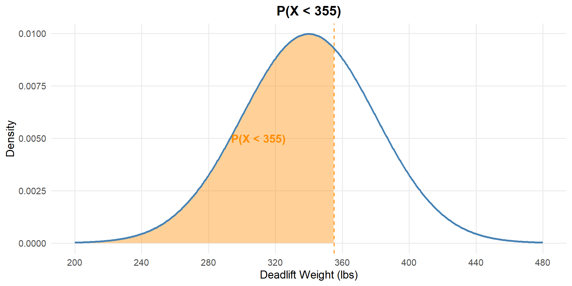
# P(X < 355)
pnorm(355, mean = 340, sd = 40)
[1] 0.6461698About 64.6% of cadets deadlift less than 355 lbs.
\(P(X = a)\) — Equal To a Single Value
What is the probability a cadet deadlifts exactly 350 lbs?
\[P(X = 350) = \int_{350}^{350} \frac{1}{40\sqrt{2\pi}} e^{-\frac{(x-340)^2}{2(40)^2}}\,dx = 0\]
The Empirical Rule (68-95-99.7)
NoteEmpirical Rule
For any normal distribution \(X \sim N(\mu, \sigma^2)\):
- 68% of values fall within \(\mu \pm 1\sigma\)
- 95% of values fall within \(\mu \pm 2\sigma\)
- 99.7% of values fall within \(\mu \pm 3\sigma\)
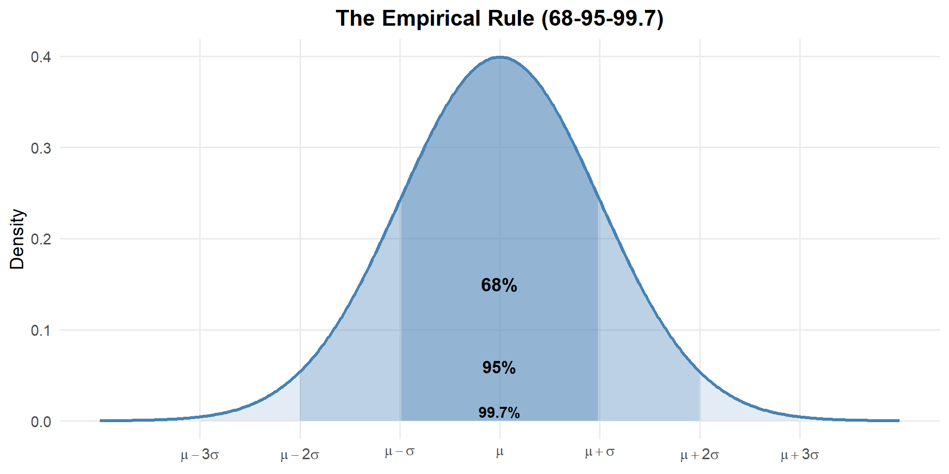
This gives us quick mental estimates before doing any calculations.
The Standard Normal Distribution
Standardization
ImportantStandardization Formula
If \(X \sim N(\mu, \sigma^2)\), then:
\[Z = \frac{X - \mu}{\sigma} \sim N(0, 1)\]
This Z-score tells you how many standard deviations \(X\) is from the mean.
- \(Z > 0\): above the mean
- \(Z < 0\): below the mean
- \(|Z| > 2\): unusually far from the mean
Why Standardize?
Standardization lets us convert any normal problem to a single reference distribution — \(N(0,1)\). This is critical because:
- The Z table (Standard Normal Table) only works for \(Z \sim N(0,1)\)
- It lets us compare values across different normal distributions
- It tells us how unusual a value is regardless of units
\[P(X \leq x) = P\left(Z \leq \frac{x - \mu}{\sigma}\right)\]
Visualizing the Transformation
Watch what happens when we take our deadlift data (\(X \sim N(340, 40^2)\)) and standardize it step by step:
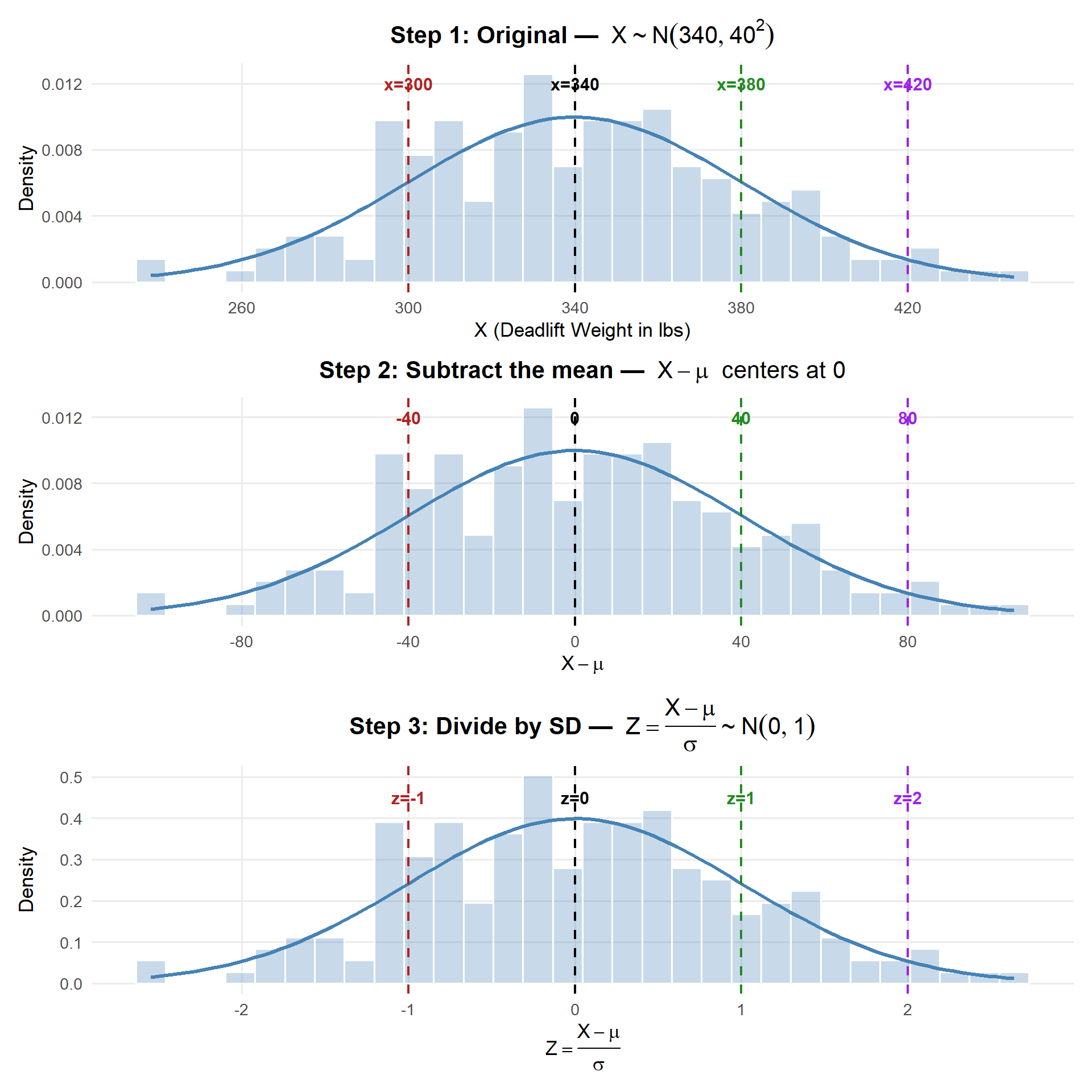
The same data, the same shape — just recentered and rescaled. A cadet who deadlifts 380 lbs is always 1 standard deviation above the mean, whether we call that value 380, 40, or 1.
Same Problems, Now with Z-Scores and the Z Table
Recall: deadlift weight \(X \sim N(\mu = 340, \sigma = 40)\). Let’s redo the same problems, but now showing the standardization step.
\(P(X < 300)\):
\[Z = \frac{300 - 340}{40} = -1\]
\[P(X < 300) = P(Z < -1) = \Phi(-1.00)\]
pnorm(300, mean = 340, sd = 40)[1] 0.1586553pnorm(-1, mean = 0, sd = 1)[1] 0.1586553Row \(-1.0\), Column \(0.00\) → \(\Phi(-1.00) =\) 0.1587
NoteZ Table
| 0.00 | 0.01 | 0.02 | 0.03 | 0.04 | 0.05 | 0.06 | 0.07 | 0.08 | 0.09 | |
|---|---|---|---|---|---|---|---|---|---|---|
| -2.0 | 0.0228 | 0.0233 | 0.0239 | 0.0244 | 0.0250 | 0.0256 | 0.0262 | 0.0268 | 0.0274 | 0.0281 |
| -1.9 | 0.0287 | 0.0294 | 0.0301 | 0.0307 | 0.0314 | 0.0322 | 0.0329 | 0.0336 | 0.0344 | 0.0351 |
| -1.8 | 0.0359 | 0.0367 | 0.0375 | 0.0384 | 0.0392 | 0.0401 | 0.0409 | 0.0418 | 0.0427 | 0.0436 |
| -1.7 | 0.0446 | 0.0455 | 0.0465 | 0.0475 | 0.0485 | 0.0495 | 0.0505 | 0.0516 | 0.0526 | 0.0537 |
| -1.6 | 0.0548 | 0.0559 | 0.0571 | 0.0582 | 0.0594 | 0.0606 | 0.0618 | 0.0630 | 0.0643 | 0.0655 |
| -1.5 | 0.0668 | 0.0681 | 0.0694 | 0.0708 | 0.0721 | 0.0735 | 0.0749 | 0.0764 | 0.0778 | 0.0793 |
| -1.4 | 0.0808 | 0.0823 | 0.0838 | 0.0853 | 0.0869 | 0.0885 | 0.0901 | 0.0918 | 0.0934 | 0.0951 |
| -1.3 | 0.0968 | 0.0985 | 0.1003 | 0.1020 | 0.1038 | 0.1056 | 0.1075 | 0.1093 | 0.1112 | 0.1131 |
| -1.2 | 0.1151 | 0.1170 | 0.1190 | 0.1210 | 0.1230 | 0.1251 | 0.1271 | 0.1292 | 0.1314 | 0.1335 |
| -1.1 | 0.1357 | 0.1379 | 0.1401 | 0.1423 | 0.1446 | 0.1469 | 0.1492 | 0.1515 | 0.1539 | 0.1562 |
| -1.0 | 0.1587 | 0.1611 | 0.1635 | 0.1660 | 0.1685 | 0.1711 | 0.1736 | 0.1762 | 0.1788 | 0.1814 |
| -0.9 | 0.1841 | 0.1867 | 0.1894 | 0.1922 | 0.1949 | 0.1977 | 0.2005 | 0.2033 | 0.2061 | 0.2090 |
| -0.8 | 0.2119 | 0.2148 | 0.2177 | 0.2206 | 0.2236 | 0.2266 | 0.2296 | 0.2327 | 0.2358 | 0.2389 |
| -0.7 | 0.2420 | 0.2451 | 0.2483 | 0.2514 | 0.2546 | 0.2578 | 0.2611 | 0.2643 | 0.2676 | 0.2709 |
| -0.6 | 0.2743 | 0.2776 | 0.2810 | 0.2843 | 0.2877 | 0.2912 | 0.2946 | 0.2981 | 0.3015 | 0.3050 |
| -0.5 | 0.3085 | 0.3121 | 0.3156 | 0.3192 | 0.3228 | 0.3264 | 0.3300 | 0.3336 | 0.3372 | 0.3409 |
| -0.4 | 0.3446 | 0.3483 | 0.3520 | 0.3557 | 0.3594 | 0.3632 | 0.3669 | 0.3707 | 0.3745 | 0.3783 |
| -0.3 | 0.3821 | 0.3859 | 0.3897 | 0.3936 | 0.3974 | 0.4013 | 0.4052 | 0.4090 | 0.4129 | 0.4168 |
| -0.2 | 0.4207 | 0.4247 | 0.4286 | 0.4325 | 0.4364 | 0.4404 | 0.4443 | 0.4483 | 0.4522 | 0.4562 |
| -0.1 | 0.4602 | 0.4641 | 0.4681 | 0.4721 | 0.4761 | 0.4801 | 0.4840 | 0.4880 | 0.4920 | 0.4960 |
| 0.0 | 0.5000 | 0.5040 | 0.5080 | 0.5120 | 0.5160 | 0.5199 | 0.5239 | 0.5279 | 0.5319 | 0.5359 |
| 0.1 | 0.5398 | 0.5438 | 0.5478 | 0.5517 | 0.5557 | 0.5596 | 0.5636 | 0.5675 | 0.5714 | 0.5753 |
| 0.2 | 0.5793 | 0.5832 | 0.5871 | 0.5910 | 0.5948 | 0.5987 | 0.6026 | 0.6064 | 0.6103 | 0.6141 |
| 0.3 | 0.6179 | 0.6217 | 0.6255 | 0.6293 | 0.6331 | 0.6368 | 0.6406 | 0.6443 | 0.6480 | 0.6517 |
| 0.4 | 0.6554 | 0.6591 | 0.6628 | 0.6664 | 0.6700 | 0.6736 | 0.6772 | 0.6808 | 0.6844 | 0.6879 |
| 0.5 | 0.6915 | 0.6950 | 0.6985 | 0.7019 | 0.7054 | 0.7088 | 0.7123 | 0.7157 | 0.7190 | 0.7224 |
| 0.6 | 0.7257 | 0.7291 | 0.7324 | 0.7357 | 0.7389 | 0.7422 | 0.7454 | 0.7486 | 0.7517 | 0.7549 |
| 0.7 | 0.7580 | 0.7611 | 0.7642 | 0.7673 | 0.7704 | 0.7734 | 0.7764 | 0.7794 | 0.7823 | 0.7852 |
| 0.8 | 0.7881 | 0.7910 | 0.7939 | 0.7967 | 0.7995 | 0.8023 | 0.8051 | 0.8078 | 0.8106 | 0.8133 |
| 0.9 | 0.8159 | 0.8186 | 0.8212 | 0.8238 | 0.8264 | 0.8289 | 0.8315 | 0.8340 | 0.8365 | 0.8389 |
| 1.0 | 0.8413 | 0.8438 | 0.8461 | 0.8485 | 0.8508 | 0.8531 | 0.8554 | 0.8577 | 0.8599 | 0.8621 |
| 1.1 | 0.8643 | 0.8665 | 0.8686 | 0.8708 | 0.8729 | 0.8749 | 0.8770 | 0.8790 | 0.8810 | 0.8830 |
| 1.2 | 0.8849 | 0.8869 | 0.8888 | 0.8907 | 0.8925 | 0.8944 | 0.8962 | 0.8980 | 0.8997 | 0.9015 |
| 1.3 | 0.9032 | 0.9049 | 0.9066 | 0.9082 | 0.9099 | 0.9115 | 0.9131 | 0.9147 | 0.9162 | 0.9177 |
| 1.4 | 0.9192 | 0.9207 | 0.9222 | 0.9236 | 0.9251 | 0.9265 | 0.9279 | 0.9292 | 0.9306 | 0.9319 |
| 1.5 | 0.9332 | 0.9345 | 0.9357 | 0.9370 | 0.9382 | 0.9394 | 0.9406 | 0.9418 | 0.9429 | 0.9441 |
| 1.6 | 0.9452 | 0.9463 | 0.9474 | 0.9484 | 0.9495 | 0.9505 | 0.9515 | 0.9525 | 0.9535 | 0.9545 |
| 1.7 | 0.9554 | 0.9564 | 0.9573 | 0.9582 | 0.9591 | 0.9599 | 0.9608 | 0.9616 | 0.9625 | 0.9633 |
| 1.8 | 0.9641 | 0.9649 | 0.9656 | 0.9664 | 0.9671 | 0.9678 | 0.9686 | 0.9693 | 0.9699 | 0.9706 |
| 1.9 | 0.9713 | 0.9719 | 0.9726 | 0.9732 | 0.9738 | 0.9744 | 0.9750 | 0.9756 | 0.9761 | 0.9767 |
| 2.0 | 0.9772 | 0.9778 | 0.9783 | 0.9788 | 0.9793 | 0.9798 | 0.9803 | 0.9808 | 0.9812 | 0.9817 |
\(P(X > 400)\):
\[Z = \frac{400 - 340}{40} = 1.5\]
\[P(X > 400) = P(Z > 1.5) = 1 - P(Z \leq 1.5) = 1 - \Phi(1.50)\]
1 - pnorm(400, mean = 340, sd = 40)[1] 0.06680721 - pnorm(1.5, mean = 0, sd = 1)[1] 0.0668072Row \(1.5\), Column \(0.00\) → \(\Phi(1.50) = 0.9332\), then \(1 - 0.9332 =\) 0.0668
NoteZ Table
| 0.00 | 0.01 | 0.02 | 0.03 | 0.04 | 0.05 | 0.06 | 0.07 | 0.08 | 0.09 | |
|---|---|---|---|---|---|---|---|---|---|---|
| -2.0 | 0.0228 | 0.0233 | 0.0239 | 0.0244 | 0.0250 | 0.0256 | 0.0262 | 0.0268 | 0.0274 | 0.0281 |
| -1.9 | 0.0287 | 0.0294 | 0.0301 | 0.0307 | 0.0314 | 0.0322 | 0.0329 | 0.0336 | 0.0344 | 0.0351 |
| -1.8 | 0.0359 | 0.0367 | 0.0375 | 0.0384 | 0.0392 | 0.0401 | 0.0409 | 0.0418 | 0.0427 | 0.0436 |
| -1.7 | 0.0446 | 0.0455 | 0.0465 | 0.0475 | 0.0485 | 0.0495 | 0.0505 | 0.0516 | 0.0526 | 0.0537 |
| -1.6 | 0.0548 | 0.0559 | 0.0571 | 0.0582 | 0.0594 | 0.0606 | 0.0618 | 0.0630 | 0.0643 | 0.0655 |
| -1.5 | 0.0668 | 0.0681 | 0.0694 | 0.0708 | 0.0721 | 0.0735 | 0.0749 | 0.0764 | 0.0778 | 0.0793 |
| -1.4 | 0.0808 | 0.0823 | 0.0838 | 0.0853 | 0.0869 | 0.0885 | 0.0901 | 0.0918 | 0.0934 | 0.0951 |
| -1.3 | 0.0968 | 0.0985 | 0.1003 | 0.1020 | 0.1038 | 0.1056 | 0.1075 | 0.1093 | 0.1112 | 0.1131 |
| -1.2 | 0.1151 | 0.1170 | 0.1190 | 0.1210 | 0.1230 | 0.1251 | 0.1271 | 0.1292 | 0.1314 | 0.1335 |
| -1.1 | 0.1357 | 0.1379 | 0.1401 | 0.1423 | 0.1446 | 0.1469 | 0.1492 | 0.1515 | 0.1539 | 0.1562 |
| -1.0 | 0.1587 | 0.1611 | 0.1635 | 0.1660 | 0.1685 | 0.1711 | 0.1736 | 0.1762 | 0.1788 | 0.1814 |
| -0.9 | 0.1841 | 0.1867 | 0.1894 | 0.1922 | 0.1949 | 0.1977 | 0.2005 | 0.2033 | 0.2061 | 0.2090 |
| -0.8 | 0.2119 | 0.2148 | 0.2177 | 0.2206 | 0.2236 | 0.2266 | 0.2296 | 0.2327 | 0.2358 | 0.2389 |
| -0.7 | 0.2420 | 0.2451 | 0.2483 | 0.2514 | 0.2546 | 0.2578 | 0.2611 | 0.2643 | 0.2676 | 0.2709 |
| -0.6 | 0.2743 | 0.2776 | 0.2810 | 0.2843 | 0.2877 | 0.2912 | 0.2946 | 0.2981 | 0.3015 | 0.3050 |
| -0.5 | 0.3085 | 0.3121 | 0.3156 | 0.3192 | 0.3228 | 0.3264 | 0.3300 | 0.3336 | 0.3372 | 0.3409 |
| -0.4 | 0.3446 | 0.3483 | 0.3520 | 0.3557 | 0.3594 | 0.3632 | 0.3669 | 0.3707 | 0.3745 | 0.3783 |
| -0.3 | 0.3821 | 0.3859 | 0.3897 | 0.3936 | 0.3974 | 0.4013 | 0.4052 | 0.4090 | 0.4129 | 0.4168 |
| -0.2 | 0.4207 | 0.4247 | 0.4286 | 0.4325 | 0.4364 | 0.4404 | 0.4443 | 0.4483 | 0.4522 | 0.4562 |
| -0.1 | 0.4602 | 0.4641 | 0.4681 | 0.4721 | 0.4761 | 0.4801 | 0.4840 | 0.4880 | 0.4920 | 0.4960 |
| 0.0 | 0.5000 | 0.5040 | 0.5080 | 0.5120 | 0.5160 | 0.5199 | 0.5239 | 0.5279 | 0.5319 | 0.5359 |
| 0.1 | 0.5398 | 0.5438 | 0.5478 | 0.5517 | 0.5557 | 0.5596 | 0.5636 | 0.5675 | 0.5714 | 0.5753 |
| 0.2 | 0.5793 | 0.5832 | 0.5871 | 0.5910 | 0.5948 | 0.5987 | 0.6026 | 0.6064 | 0.6103 | 0.6141 |
| 0.3 | 0.6179 | 0.6217 | 0.6255 | 0.6293 | 0.6331 | 0.6368 | 0.6406 | 0.6443 | 0.6480 | 0.6517 |
| 0.4 | 0.6554 | 0.6591 | 0.6628 | 0.6664 | 0.6700 | 0.6736 | 0.6772 | 0.6808 | 0.6844 | 0.6879 |
| 0.5 | 0.6915 | 0.6950 | 0.6985 | 0.7019 | 0.7054 | 0.7088 | 0.7123 | 0.7157 | 0.7190 | 0.7224 |
| 0.6 | 0.7257 | 0.7291 | 0.7324 | 0.7357 | 0.7389 | 0.7422 | 0.7454 | 0.7486 | 0.7517 | 0.7549 |
| 0.7 | 0.7580 | 0.7611 | 0.7642 | 0.7673 | 0.7704 | 0.7734 | 0.7764 | 0.7794 | 0.7823 | 0.7852 |
| 0.8 | 0.7881 | 0.7910 | 0.7939 | 0.7967 | 0.7995 | 0.8023 | 0.8051 | 0.8078 | 0.8106 | 0.8133 |
| 0.9 | 0.8159 | 0.8186 | 0.8212 | 0.8238 | 0.8264 | 0.8289 | 0.8315 | 0.8340 | 0.8365 | 0.8389 |
| 1.0 | 0.8413 | 0.8438 | 0.8461 | 0.8485 | 0.8508 | 0.8531 | 0.8554 | 0.8577 | 0.8599 | 0.8621 |
| 1.1 | 0.8643 | 0.8665 | 0.8686 | 0.8708 | 0.8729 | 0.8749 | 0.8770 | 0.8790 | 0.8810 | 0.8830 |
| 1.2 | 0.8849 | 0.8869 | 0.8888 | 0.8907 | 0.8925 | 0.8944 | 0.8962 | 0.8980 | 0.8997 | 0.9015 |
| 1.3 | 0.9032 | 0.9049 | 0.9066 | 0.9082 | 0.9099 | 0.9115 | 0.9131 | 0.9147 | 0.9162 | 0.9177 |
| 1.4 | 0.9192 | 0.9207 | 0.9222 | 0.9236 | 0.9251 | 0.9265 | 0.9279 | 0.9292 | 0.9306 | 0.9319 |
| 1.5 | 0.9332 | 0.9345 | 0.9357 | 0.9370 | 0.9382 | 0.9394 | 0.9406 | 0.9418 | 0.9429 | 0.9441 |
| 1.6 | 0.9452 | 0.9463 | 0.9474 | 0.9484 | 0.9495 | 0.9505 | 0.9515 | 0.9525 | 0.9535 | 0.9545 |
| 1.7 | 0.9554 | 0.9564 | 0.9573 | 0.9582 | 0.9591 | 0.9599 | 0.9608 | 0.9616 | 0.9625 | 0.9633 |
| 1.8 | 0.9641 | 0.9649 | 0.9656 | 0.9664 | 0.9671 | 0.9678 | 0.9686 | 0.9693 | 0.9699 | 0.9706 |
| 1.9 | 0.9713 | 0.9719 | 0.9726 | 0.9732 | 0.9738 | 0.9744 | 0.9750 | 0.9756 | 0.9761 | 0.9767 |
| 2.0 | 0.9772 | 0.9778 | 0.9783 | 0.9788 | 0.9793 | 0.9798 | 0.9803 | 0.9808 | 0.9812 | 0.9817 |
\(P(300 < X < 380)\):
\[Z_1 = \frac{300 - 340}{40} = -1, \quad Z_2 = \frac{380 - 340}{40} = 1\]
\[P(300 < X < 380) = P(-1 < Z < 1) = \Phi(1.00) - \Phi(-1.00)\]
pnorm(380, mean = 340, sd = 40) - pnorm(300, mean = 340, sd = 40)[1] 0.6826895pnorm(1, mean = 0, sd = 1) - pnorm(-1, mean = 0, sd = 1)[1] 0.6826895\(\Phi(1.00) = 0.8413\) and \(\Phi(-1.00) = 0.1587\), then \(0.8413 - 0.1587 =\) 0.6826
NoteZ Table
| 0.00 | 0.01 | 0.02 | 0.03 | 0.04 | 0.05 | 0.06 | 0.07 | 0.08 | 0.09 | |
|---|---|---|---|---|---|---|---|---|---|---|
| -2.0 | 0.0228 | 0.0233 | 0.0239 | 0.0244 | 0.0250 | 0.0256 | 0.0262 | 0.0268 | 0.0274 | 0.0281 |
| -1.9 | 0.0287 | 0.0294 | 0.0301 | 0.0307 | 0.0314 | 0.0322 | 0.0329 | 0.0336 | 0.0344 | 0.0351 |
| -1.8 | 0.0359 | 0.0367 | 0.0375 | 0.0384 | 0.0392 | 0.0401 | 0.0409 | 0.0418 | 0.0427 | 0.0436 |
| -1.7 | 0.0446 | 0.0455 | 0.0465 | 0.0475 | 0.0485 | 0.0495 | 0.0505 | 0.0516 | 0.0526 | 0.0537 |
| -1.6 | 0.0548 | 0.0559 | 0.0571 | 0.0582 | 0.0594 | 0.0606 | 0.0618 | 0.0630 | 0.0643 | 0.0655 |
| -1.5 | 0.0668 | 0.0681 | 0.0694 | 0.0708 | 0.0721 | 0.0735 | 0.0749 | 0.0764 | 0.0778 | 0.0793 |
| -1.4 | 0.0808 | 0.0823 | 0.0838 | 0.0853 | 0.0869 | 0.0885 | 0.0901 | 0.0918 | 0.0934 | 0.0951 |
| -1.3 | 0.0968 | 0.0985 | 0.1003 | 0.1020 | 0.1038 | 0.1056 | 0.1075 | 0.1093 | 0.1112 | 0.1131 |
| -1.2 | 0.1151 | 0.1170 | 0.1190 | 0.1210 | 0.1230 | 0.1251 | 0.1271 | 0.1292 | 0.1314 | 0.1335 |
| -1.1 | 0.1357 | 0.1379 | 0.1401 | 0.1423 | 0.1446 | 0.1469 | 0.1492 | 0.1515 | 0.1539 | 0.1562 |
| -1.0 | 0.1587 | 0.1611 | 0.1635 | 0.1660 | 0.1685 | 0.1711 | 0.1736 | 0.1762 | 0.1788 | 0.1814 |
| -0.9 | 0.1841 | 0.1867 | 0.1894 | 0.1922 | 0.1949 | 0.1977 | 0.2005 | 0.2033 | 0.2061 | 0.2090 |
| -0.8 | 0.2119 | 0.2148 | 0.2177 | 0.2206 | 0.2236 | 0.2266 | 0.2296 | 0.2327 | 0.2358 | 0.2389 |
| -0.7 | 0.2420 | 0.2451 | 0.2483 | 0.2514 | 0.2546 | 0.2578 | 0.2611 | 0.2643 | 0.2676 | 0.2709 |
| -0.6 | 0.2743 | 0.2776 | 0.2810 | 0.2843 | 0.2877 | 0.2912 | 0.2946 | 0.2981 | 0.3015 | 0.3050 |
| -0.5 | 0.3085 | 0.3121 | 0.3156 | 0.3192 | 0.3228 | 0.3264 | 0.3300 | 0.3336 | 0.3372 | 0.3409 |
| -0.4 | 0.3446 | 0.3483 | 0.3520 | 0.3557 | 0.3594 | 0.3632 | 0.3669 | 0.3707 | 0.3745 | 0.3783 |
| -0.3 | 0.3821 | 0.3859 | 0.3897 | 0.3936 | 0.3974 | 0.4013 | 0.4052 | 0.4090 | 0.4129 | 0.4168 |
| -0.2 | 0.4207 | 0.4247 | 0.4286 | 0.4325 | 0.4364 | 0.4404 | 0.4443 | 0.4483 | 0.4522 | 0.4562 |
| -0.1 | 0.4602 | 0.4641 | 0.4681 | 0.4721 | 0.4761 | 0.4801 | 0.4840 | 0.4880 | 0.4920 | 0.4960 |
| 0.0 | 0.5000 | 0.5040 | 0.5080 | 0.5120 | 0.5160 | 0.5199 | 0.5239 | 0.5279 | 0.5319 | 0.5359 |
| 0.1 | 0.5398 | 0.5438 | 0.5478 | 0.5517 | 0.5557 | 0.5596 | 0.5636 | 0.5675 | 0.5714 | 0.5753 |
| 0.2 | 0.5793 | 0.5832 | 0.5871 | 0.5910 | 0.5948 | 0.5987 | 0.6026 | 0.6064 | 0.6103 | 0.6141 |
| 0.3 | 0.6179 | 0.6217 | 0.6255 | 0.6293 | 0.6331 | 0.6368 | 0.6406 | 0.6443 | 0.6480 | 0.6517 |
| 0.4 | 0.6554 | 0.6591 | 0.6628 | 0.6664 | 0.6700 | 0.6736 | 0.6772 | 0.6808 | 0.6844 | 0.6879 |
| 0.5 | 0.6915 | 0.6950 | 0.6985 | 0.7019 | 0.7054 | 0.7088 | 0.7123 | 0.7157 | 0.7190 | 0.7224 |
| 0.6 | 0.7257 | 0.7291 | 0.7324 | 0.7357 | 0.7389 | 0.7422 | 0.7454 | 0.7486 | 0.7517 | 0.7549 |
| 0.7 | 0.7580 | 0.7611 | 0.7642 | 0.7673 | 0.7704 | 0.7734 | 0.7764 | 0.7794 | 0.7823 | 0.7852 |
| 0.8 | 0.7881 | 0.7910 | 0.7939 | 0.7967 | 0.7995 | 0.8023 | 0.8051 | 0.8078 | 0.8106 | 0.8133 |
| 0.9 | 0.8159 | 0.8186 | 0.8212 | 0.8238 | 0.8264 | 0.8289 | 0.8315 | 0.8340 | 0.8365 | 0.8389 |
| 1.0 | 0.8413 | 0.8438 | 0.8461 | 0.8485 | 0.8508 | 0.8531 | 0.8554 | 0.8577 | 0.8599 | 0.8621 |
| 1.1 | 0.8643 | 0.8665 | 0.8686 | 0.8708 | 0.8729 | 0.8749 | 0.8770 | 0.8790 | 0.8810 | 0.8830 |
| 1.2 | 0.8849 | 0.8869 | 0.8888 | 0.8907 | 0.8925 | 0.8944 | 0.8962 | 0.8980 | 0.8997 | 0.9015 |
| 1.3 | 0.9032 | 0.9049 | 0.9066 | 0.9082 | 0.9099 | 0.9115 | 0.9131 | 0.9147 | 0.9162 | 0.9177 |
| 1.4 | 0.9192 | 0.9207 | 0.9222 | 0.9236 | 0.9251 | 0.9265 | 0.9279 | 0.9292 | 0.9306 | 0.9319 |
| 1.5 | 0.9332 | 0.9345 | 0.9357 | 0.9370 | 0.9382 | 0.9394 | 0.9406 | 0.9418 | 0.9429 | 0.9441 |
| 1.6 | 0.9452 | 0.9463 | 0.9474 | 0.9484 | 0.9495 | 0.9505 | 0.9515 | 0.9525 | 0.9535 | 0.9545 |
| 1.7 | 0.9554 | 0.9564 | 0.9573 | 0.9582 | 0.9591 | 0.9599 | 0.9608 | 0.9616 | 0.9625 | 0.9633 |
| 1.8 | 0.9641 | 0.9649 | 0.9656 | 0.9664 | 0.9671 | 0.9678 | 0.9686 | 0.9693 | 0.9699 | 0.9706 |
| 1.9 | 0.9713 | 0.9719 | 0.9726 | 0.9732 | 0.9738 | 0.9744 | 0.9750 | 0.9756 | 0.9761 | 0.9767 |
| 2.0 | 0.9772 | 0.9778 | 0.9783 | 0.9788 | 0.9793 | 0.9798 | 0.9803 | 0.9808 | 0.9812 | 0.9817 |
\(P(X < 355)\):
\[Z = \frac{355 - 340}{40} = \frac{15}{40} = 0.375 \approx 0.38\]
\[P(X < 355) = P(Z < 0.38) = \Phi(0.38)\]
pnorm(355, mean = 340, sd = 40)[1] 0.6461698pnorm(0.38, mean = 0, sd = 1)[1] 0.6480273Row \(0.3\), Column \(0.08\) → \(\Phi(0.38) =\) 0.6480
NoteZ Table
| 0.00 | 0.01 | 0.02 | 0.03 | 0.04 | 0.05 | 0.06 | 0.07 | 0.08 | 0.09 | |
|---|---|---|---|---|---|---|---|---|---|---|
| -2.0 | 0.0228 | 0.0233 | 0.0239 | 0.0244 | 0.0250 | 0.0256 | 0.0262 | 0.0268 | 0.0274 | 0.0281 |
| -1.9 | 0.0287 | 0.0294 | 0.0301 | 0.0307 | 0.0314 | 0.0322 | 0.0329 | 0.0336 | 0.0344 | 0.0351 |
| -1.8 | 0.0359 | 0.0367 | 0.0375 | 0.0384 | 0.0392 | 0.0401 | 0.0409 | 0.0418 | 0.0427 | 0.0436 |
| -1.7 | 0.0446 | 0.0455 | 0.0465 | 0.0475 | 0.0485 | 0.0495 | 0.0505 | 0.0516 | 0.0526 | 0.0537 |
| -1.6 | 0.0548 | 0.0559 | 0.0571 | 0.0582 | 0.0594 | 0.0606 | 0.0618 | 0.0630 | 0.0643 | 0.0655 |
| -1.5 | 0.0668 | 0.0681 | 0.0694 | 0.0708 | 0.0721 | 0.0735 | 0.0749 | 0.0764 | 0.0778 | 0.0793 |
| -1.4 | 0.0808 | 0.0823 | 0.0838 | 0.0853 | 0.0869 | 0.0885 | 0.0901 | 0.0918 | 0.0934 | 0.0951 |
| -1.3 | 0.0968 | 0.0985 | 0.1003 | 0.1020 | 0.1038 | 0.1056 | 0.1075 | 0.1093 | 0.1112 | 0.1131 |
| -1.2 | 0.1151 | 0.1170 | 0.1190 | 0.1210 | 0.1230 | 0.1251 | 0.1271 | 0.1292 | 0.1314 | 0.1335 |
| -1.1 | 0.1357 | 0.1379 | 0.1401 | 0.1423 | 0.1446 | 0.1469 | 0.1492 | 0.1515 | 0.1539 | 0.1562 |
| -1.0 | 0.1587 | 0.1611 | 0.1635 | 0.1660 | 0.1685 | 0.1711 | 0.1736 | 0.1762 | 0.1788 | 0.1814 |
| -0.9 | 0.1841 | 0.1867 | 0.1894 | 0.1922 | 0.1949 | 0.1977 | 0.2005 | 0.2033 | 0.2061 | 0.2090 |
| -0.8 | 0.2119 | 0.2148 | 0.2177 | 0.2206 | 0.2236 | 0.2266 | 0.2296 | 0.2327 | 0.2358 | 0.2389 |
| -0.7 | 0.2420 | 0.2451 | 0.2483 | 0.2514 | 0.2546 | 0.2578 | 0.2611 | 0.2643 | 0.2676 | 0.2709 |
| -0.6 | 0.2743 | 0.2776 | 0.2810 | 0.2843 | 0.2877 | 0.2912 | 0.2946 | 0.2981 | 0.3015 | 0.3050 |
| -0.5 | 0.3085 | 0.3121 | 0.3156 | 0.3192 | 0.3228 | 0.3264 | 0.3300 | 0.3336 | 0.3372 | 0.3409 |
| -0.4 | 0.3446 | 0.3483 | 0.3520 | 0.3557 | 0.3594 | 0.3632 | 0.3669 | 0.3707 | 0.3745 | 0.3783 |
| -0.3 | 0.3821 | 0.3859 | 0.3897 | 0.3936 | 0.3974 | 0.4013 | 0.4052 | 0.4090 | 0.4129 | 0.4168 |
| -0.2 | 0.4207 | 0.4247 | 0.4286 | 0.4325 | 0.4364 | 0.4404 | 0.4443 | 0.4483 | 0.4522 | 0.4562 |
| -0.1 | 0.4602 | 0.4641 | 0.4681 | 0.4721 | 0.4761 | 0.4801 | 0.4840 | 0.4880 | 0.4920 | 0.4960 |
| 0.0 | 0.5000 | 0.5040 | 0.5080 | 0.5120 | 0.5160 | 0.5199 | 0.5239 | 0.5279 | 0.5319 | 0.5359 |
| 0.1 | 0.5398 | 0.5438 | 0.5478 | 0.5517 | 0.5557 | 0.5596 | 0.5636 | 0.5675 | 0.5714 | 0.5753 |
| 0.2 | 0.5793 | 0.5832 | 0.5871 | 0.5910 | 0.5948 | 0.5987 | 0.6026 | 0.6064 | 0.6103 | 0.6141 |
| 0.3 | 0.6179 | 0.6217 | 0.6255 | 0.6293 | 0.6331 | 0.6368 | 0.6406 | 0.6443 | 0.6480 | 0.6517 |
| 0.4 | 0.6554 | 0.6591 | 0.6628 | 0.6664 | 0.6700 | 0.6736 | 0.6772 | 0.6808 | 0.6844 | 0.6879 |
| 0.5 | 0.6915 | 0.6950 | 0.6985 | 0.7019 | 0.7054 | 0.7088 | 0.7123 | 0.7157 | 0.7190 | 0.7224 |
| 0.6 | 0.7257 | 0.7291 | 0.7324 | 0.7357 | 0.7389 | 0.7422 | 0.7454 | 0.7486 | 0.7517 | 0.7549 |
| 0.7 | 0.7580 | 0.7611 | 0.7642 | 0.7673 | 0.7704 | 0.7734 | 0.7764 | 0.7794 | 0.7823 | 0.7852 |
| 0.8 | 0.7881 | 0.7910 | 0.7939 | 0.7967 | 0.7995 | 0.8023 | 0.8051 | 0.8078 | 0.8106 | 0.8133 |
| 0.9 | 0.8159 | 0.8186 | 0.8212 | 0.8238 | 0.8264 | 0.8289 | 0.8315 | 0.8340 | 0.8365 | 0.8389 |
| 1.0 | 0.8413 | 0.8438 | 0.8461 | 0.8485 | 0.8508 | 0.8531 | 0.8554 | 0.8577 | 0.8599 | 0.8621 |
| 1.1 | 0.8643 | 0.8665 | 0.8686 | 0.8708 | 0.8729 | 0.8749 | 0.8770 | 0.8790 | 0.8810 | 0.8830 |
| 1.2 | 0.8849 | 0.8869 | 0.8888 | 0.8907 | 0.8925 | 0.8944 | 0.8962 | 0.8980 | 0.8997 | 0.9015 |
| 1.3 | 0.9032 | 0.9049 | 0.9066 | 0.9082 | 0.9099 | 0.9115 | 0.9131 | 0.9147 | 0.9162 | 0.9177 |
| 1.4 | 0.9192 | 0.9207 | 0.9222 | 0.9236 | 0.9251 | 0.9265 | 0.9279 | 0.9292 | 0.9306 | 0.9319 |
| 1.5 | 0.9332 | 0.9345 | 0.9357 | 0.9370 | 0.9382 | 0.9394 | 0.9406 | 0.9418 | 0.9429 | 0.9441 |
| 1.6 | 0.9452 | 0.9463 | 0.9474 | 0.9484 | 0.9495 | 0.9505 | 0.9515 | 0.9525 | 0.9535 | 0.9545 |
| 1.7 | 0.9554 | 0.9564 | 0.9573 | 0.9582 | 0.9591 | 0.9599 | 0.9608 | 0.9616 | 0.9625 | 0.9633 |
| 1.8 | 0.9641 | 0.9649 | 0.9656 | 0.9664 | 0.9671 | 0.9678 | 0.9686 | 0.9693 | 0.9699 | 0.9706 |
| 1.9 | 0.9713 | 0.9719 | 0.9726 | 0.9732 | 0.9738 | 0.9744 | 0.9750 | 0.9756 | 0.9761 | 0.9767 |
| 2.0 | 0.9772 | 0.9778 | 0.9783 | 0.9788 | 0.9793 | 0.9798 | 0.9803 | 0.9808 | 0.9812 | 0.9817 |
\(P(X = 350)\):
\[Z = \frac{350 - 340}{40} = 0.25\]
\[P(X = 350) = P(Z = 0.25) = 0\]
Still zero. For continuous RVs, the probability at any single point is always zero.
ImportantZ Table Patterns Summary
| Problem Type | Formula | Z Table Steps |
|---|---|---|
| \(P(X < a)\) | \(\Phi(z)\) | Standardize, look up \(z\) directly |
| \(P(X > a)\) | \(1 - \Phi(z)\) | Look up \(z\), subtract from 1 |
| \(P(a < X < b)\) | \(\Phi(z_2) - \Phi(z_1)\) | Look up both, subtract |
The Quantile Function (Going Backwards)
From Probability to Value
So far we’ve gone forward: given a value \(x\), find the probability. The quantile function goes backwards: given a probability, find the value.
ImportantThe Quantile Function (Inverse Normal)
The \(p\)-th quantile (or \(100p\)-th percentile) is the value \(x\) such that:
\[P(X \leq x) = p\]
In R: qnorm(p, mean, sd) gives the value \(x\) where \(P(X \leq x) = p\).
Quantile Example 1
What deadlift weight marks the top 10% of cadets?
We need \(x\) such that \(P(X \leq x) = 0.90\) (top 10% means 90th percentile).
qnorm(0.90, mean = 340, sd = 40)[1] 391.2621A cadet needs to deadlift about 391 lbs to be in the top 10%.
Quantile Example 2: Middle 90% Range
What range contains the middle 90% of cadets?
The middle 90% leaves 5% in each tail: find the 5th and 95th percentiles.
qnorm(0.05, mean = 340, sd = 40)[1] 274.2059qnorm(0.95, mean = 340, sd = 40)[1] 405.7941The middle 90% of cadets deadlift between about 274 lbs and 406 lbs.
Quantile Example 3: Using Standard Normal
A cadet wants to be in the top 25% of deadlifters. What weight do they need to hit?
Top 25% means we need the 75th percentile: \(P(X \leq x) = 0.75\).
Step 1: Write out what we need:
\[P(X \leq x) = 0.75\]
Step 2: Standardize:
\[P\left(\frac{X - \mu}{\sigma} \leq \frac{x - \mu}{\sigma}\right) = 0.75\]
\[P\left(Z \leq \frac{x - 340}{40}\right) = 0.75\]
Step 3: Find the z-value where \(\Phi(z) = 0.75\):
qnorm(0.75)[1] 0.6744898
NoteZ Table
| 0.00 | 0.01 | 0.02 | 0.03 | 0.04 | 0.05 | 0.06 | 0.07 | 0.08 | 0.09 | |
|---|---|---|---|---|---|---|---|---|---|---|
| -2.0 | 0.0228 | 0.0233 | 0.0239 | 0.0244 | 0.0250 | 0.0256 | 0.0262 | 0.0268 | 0.0274 | 0.0281 |
| -1.9 | 0.0287 | 0.0294 | 0.0301 | 0.0307 | 0.0314 | 0.0322 | 0.0329 | 0.0336 | 0.0344 | 0.0351 |
| -1.8 | 0.0359 | 0.0367 | 0.0375 | 0.0384 | 0.0392 | 0.0401 | 0.0409 | 0.0418 | 0.0427 | 0.0436 |
| -1.7 | 0.0446 | 0.0455 | 0.0465 | 0.0475 | 0.0485 | 0.0495 | 0.0505 | 0.0516 | 0.0526 | 0.0537 |
| -1.6 | 0.0548 | 0.0559 | 0.0571 | 0.0582 | 0.0594 | 0.0606 | 0.0618 | 0.0630 | 0.0643 | 0.0655 |
| -1.5 | 0.0668 | 0.0681 | 0.0694 | 0.0708 | 0.0721 | 0.0735 | 0.0749 | 0.0764 | 0.0778 | 0.0793 |
| -1.4 | 0.0808 | 0.0823 | 0.0838 | 0.0853 | 0.0869 | 0.0885 | 0.0901 | 0.0918 | 0.0934 | 0.0951 |
| -1.3 | 0.0968 | 0.0985 | 0.1003 | 0.1020 | 0.1038 | 0.1056 | 0.1075 | 0.1093 | 0.1112 | 0.1131 |
| -1.2 | 0.1151 | 0.1170 | 0.1190 | 0.1210 | 0.1230 | 0.1251 | 0.1271 | 0.1292 | 0.1314 | 0.1335 |
| -1.1 | 0.1357 | 0.1379 | 0.1401 | 0.1423 | 0.1446 | 0.1469 | 0.1492 | 0.1515 | 0.1539 | 0.1562 |
| -1.0 | 0.1587 | 0.1611 | 0.1635 | 0.1660 | 0.1685 | 0.1711 | 0.1736 | 0.1762 | 0.1788 | 0.1814 |
| -0.9 | 0.1841 | 0.1867 | 0.1894 | 0.1922 | 0.1949 | 0.1977 | 0.2005 | 0.2033 | 0.2061 | 0.2090 |
| -0.8 | 0.2119 | 0.2148 | 0.2177 | 0.2206 | 0.2236 | 0.2266 | 0.2296 | 0.2327 | 0.2358 | 0.2389 |
| -0.7 | 0.2420 | 0.2451 | 0.2483 | 0.2514 | 0.2546 | 0.2578 | 0.2611 | 0.2643 | 0.2676 | 0.2709 |
| -0.6 | 0.2743 | 0.2776 | 0.2810 | 0.2843 | 0.2877 | 0.2912 | 0.2946 | 0.2981 | 0.3015 | 0.3050 |
| -0.5 | 0.3085 | 0.3121 | 0.3156 | 0.3192 | 0.3228 | 0.3264 | 0.3300 | 0.3336 | 0.3372 | 0.3409 |
| -0.4 | 0.3446 | 0.3483 | 0.3520 | 0.3557 | 0.3594 | 0.3632 | 0.3669 | 0.3707 | 0.3745 | 0.3783 |
| -0.3 | 0.3821 | 0.3859 | 0.3897 | 0.3936 | 0.3974 | 0.4013 | 0.4052 | 0.4090 | 0.4129 | 0.4168 |
| -0.2 | 0.4207 | 0.4247 | 0.4286 | 0.4325 | 0.4364 | 0.4404 | 0.4443 | 0.4483 | 0.4522 | 0.4562 |
| -0.1 | 0.4602 | 0.4641 | 0.4681 | 0.4721 | 0.4761 | 0.4801 | 0.4840 | 0.4880 | 0.4920 | 0.4960 |
| 0.0 | 0.5000 | 0.5040 | 0.5080 | 0.5120 | 0.5160 | 0.5199 | 0.5239 | 0.5279 | 0.5319 | 0.5359 |
| 0.1 | 0.5398 | 0.5438 | 0.5478 | 0.5517 | 0.5557 | 0.5596 | 0.5636 | 0.5675 | 0.5714 | 0.5753 |
| 0.2 | 0.5793 | 0.5832 | 0.5871 | 0.5910 | 0.5948 | 0.5987 | 0.6026 | 0.6064 | 0.6103 | 0.6141 |
| 0.3 | 0.6179 | 0.6217 | 0.6255 | 0.6293 | 0.6331 | 0.6368 | 0.6406 | 0.6443 | 0.6480 | 0.6517 |
| 0.4 | 0.6554 | 0.6591 | 0.6628 | 0.6664 | 0.6700 | 0.6736 | 0.6772 | 0.6808 | 0.6844 | 0.6879 |
| 0.5 | 0.6915 | 0.6950 | 0.6985 | 0.7019 | 0.7054 | 0.7088 | 0.7123 | 0.7157 | 0.7190 | 0.7224 |
| 0.6 | 0.7257 | 0.7291 | 0.7324 | 0.7357 | 0.7389 | 0.7422 | 0.7454 | 0.7486 | 0.7517 | 0.7549 |
| 0.7 | 0.7580 | 0.7611 | 0.7642 | 0.7673 | 0.7704 | 0.7734 | 0.7764 | 0.7794 | 0.7823 | 0.7852 |
| 0.8 | 0.7881 | 0.7910 | 0.7939 | 0.7967 | 0.7995 | 0.8023 | 0.8051 | 0.8078 | 0.8106 | 0.8133 |
| 0.9 | 0.8159 | 0.8186 | 0.8212 | 0.8238 | 0.8264 | 0.8289 | 0.8315 | 0.8340 | 0.8365 | 0.8389 |
| 1.0 | 0.8413 | 0.8438 | 0.8461 | 0.8485 | 0.8508 | 0.8531 | 0.8554 | 0.8577 | 0.8599 | 0.8621 |
| 1.1 | 0.8643 | 0.8665 | 0.8686 | 0.8708 | 0.8729 | 0.8749 | 0.8770 | 0.8790 | 0.8810 | 0.8830 |
| 1.2 | 0.8849 | 0.8869 | 0.8888 | 0.8907 | 0.8925 | 0.8944 | 0.8962 | 0.8980 | 0.8997 | 0.9015 |
| 1.3 | 0.9032 | 0.9049 | 0.9066 | 0.9082 | 0.9099 | 0.9115 | 0.9131 | 0.9147 | 0.9162 | 0.9177 |
| 1.4 | 0.9192 | 0.9207 | 0.9222 | 0.9236 | 0.9251 | 0.9265 | 0.9279 | 0.9292 | 0.9306 | 0.9319 |
| 1.5 | 0.9332 | 0.9345 | 0.9357 | 0.9370 | 0.9382 | 0.9394 | 0.9406 | 0.9418 | 0.9429 | 0.9441 |
| 1.6 | 0.9452 | 0.9463 | 0.9474 | 0.9484 | 0.9495 | 0.9505 | 0.9515 | 0.9525 | 0.9535 | 0.9545 |
| 1.7 | 0.9554 | 0.9564 | 0.9573 | 0.9582 | 0.9591 | 0.9599 | 0.9608 | 0.9616 | 0.9625 | 0.9633 |
| 1.8 | 0.9641 | 0.9649 | 0.9656 | 0.9664 | 0.9671 | 0.9678 | 0.9686 | 0.9693 | 0.9699 | 0.9706 |
| 1.9 | 0.9713 | 0.9719 | 0.9726 | 0.9732 | 0.9738 | 0.9744 | 0.9750 | 0.9756 | 0.9761 | 0.9767 |
| 2.0 | 0.9772 | 0.9778 | 0.9783 | 0.9788 | 0.9793 | 0.9798 | 0.9803 | 0.9808 | 0.9812 | 0.9817 |
So \(\frac{x - 340}{40} = 0.6745\).
Step 4: Solve for \(x\):
\[x = 340 + (0.6745)(40) = 340 + 26.98 = 366.98\]
Verify by doing it in one step with qnorm:
qnorm(0.75, mean = 340, sd = 40)[1] 366.9796A cadet needs to deadlift about 367 lbs to be in the top 25%.
ImportantTwo Directions
| Direction | Given | Find | R Function |
|---|---|---|---|
| Forward | Value \(x\) | Probability \(P(X \leq x)\) | pnorm(x, mean, sd) |
| Backward | Probability \(p\) | Value \(x\) | qnorm(p, mean, sd) |
Practice: Z Table Lookup
Try these lookups on the Z table and then verify with R.
NoteQuick Practice
- \(P(Z \leq 1.96) =\)
- \(P(Z \leq -0.50) =\)
- \(P(Z > 1.15) =\)
- \(P(-1.50 \leq Z \leq 0.75) =\)
- \(P(Z \leq -1.23) =\)
TipQuick Practice Answers
# 1. P(Z ≤ 1.96) — Row 1.9, Col 0.06
pnorm(1.96)      # 0.9750
[1] 0.9750021# 2. P(Z ≤ -0.50) — Row -0.5, Col 0.00
pnorm(-0.50) # 0.3085[1] 0.3085375# 3. P(Z > 1.15) = 1 - P(Z ≤ 1.15) — Row 1.1, Col 0.05
1 - pnorm(1.15) # 0.1251[1] 0.1250719# 4. P(-1.50 ≤ Z ≤ 0.75) = Φ(0.75) - Φ(-1.50)
pnorm(0.75) - pnorm(-1.50) # 0.7066[1] 0.7065654# 5. P(Z ≤ -1.23) — Row -1.2, Col 0.03
pnorm(-1.23) # 0.1093[1] 0.1093486Discrete vs. Continuous Distributions: The Complete Picture
NoteAll Distributions So Far
| General Discrete | Binomial | Poisson | General Continuous | Normal | |
|---|---|---|---|---|---|
| Type | Discrete | Discrete | Discrete | Continuous | Continuous |
| Notation | PMF table | \(X \sim \text{Bin}(n, p)\) | \(X \sim \text{Pois}(\lambda)\) | PDF \(f(x)\) | \(X \sim N(\mu, \sigma^2)\) |
| Parameters | Given by table | \(n, p\) | \(\lambda\) | Given by \(f(x)\) | \(\mu, \sigma\) |
| Mean | \(\sum x \cdot p(x)\) | \(np\) | \(\lambda\) | \(\int x \cdot f(x)\,dx\) | \(\mu\) |
| Variance | \(E(X^2) - \mu^2\) | \(np(1-p)\) | \(\lambda\) | \(E(X^2) - \mu^2\) | \(\sigma^2\) |
| SD | \(\sqrt{Var(X)}\) | \(\sqrt{np(1-p)}\) | \(\sqrt{\lambda}\) | \(\sqrt{Var(X)}\) | \(\sigma\) |
| R PMF/PDF | manual | dbinom |
dpois |
manual | dnorm |
| R CDF | cumsum |
pbinom |
ppois |
manual | pnorm |
| R Quantile | — | qbinom |
qpois |
— | qnorm |
Board Problems
Problem 1: APFT Run Times
The 2-mile run times (in minutes) for cadets at West Point follow a normal distribution with \(\mu = 14.5\) and \(\sigma = 1.8\).
NoteQuestions
What proportion of cadets finish in under 13 minutes?
What proportion of cadets take longer than 17 minutes?
What proportion of cadets finish between 13 and 16 minutes?
What run time marks the fastest 5% of cadets?
A cadet finishes in 11.2 minutes. How unusual is this? Find their Z-score and interpret.
TipAnswers
- \(P(X < 13) = P\left(Z < \frac{13 - 14.5}{1.8}\right) = P(Z < -0.833)\)
[1] 0.2023284About 20.2% of cadets finish in under 13 minutes.
- \(P(X > 17) = 1 - P(X \leq 17)\)
[1] 0.08243327About 8.2% of cadets take longer than 17 minutes.
- \(P(13 \leq X \leq 16) = P(X \leq 16) - P(X \leq 13)\)
[1] 0.5953432About 59.6% of cadets finish between 13 and 16 minutes.
- We need \(x\) such that \(P(X \leq x) = 0.05\):
[1] 11.53926The fastest 5% finish in under about 11.5 minutes.
- \(Z = \frac{11.2 - 14.5}{1.8} = \frac{-3.3}{1.8} = -1.83\)
This cadet is 1.83 standard deviations below the mean — faster than most. \(P(Z < -1.83) \approx 0.034\), so only about 3.4% of cadets are this fast or faster. Unusual but not extraordinary.
Problem 2: Ammunition Weight
A crate of 5.56mm ammunition has a nominal weight that is normally distributed with \(\mu = 32.0\) lbs and \(\sigma = 0.5\) lbs. Quality control rejects any crate outside the range 31.0 to 33.0 lbs.
NoteQuestions
What proportion of crates pass quality control?
What proportion are rejected for being too heavy?
The unit wants to tighten standards so that only 90% of crates pass. What symmetric range around the mean should they use?
A supply sergeant receives a crate weighing 33.2 lbs. What is the Z-score? Should they be concerned?
TipAnswers
- \(P(31 \leq X \leq 33) = P(X \leq 33) - P(X \leq 31)\)
[1] 0.9544997About 95.4% of crates pass — this is \(\mu \pm 2\sigma\), consistent with the empirical rule.
- \(P(X > 33)\)
[1] 0.02275013About 2.3% are rejected for being too heavy.
- We need values \(a\) and \(b\) symmetric about 32 such that \(P(a \leq X \leq b) = 0.90\). This leaves 5% in each tail.
[1] 31.17757[1] 32.82243The range should be approximately 31.18 to 32.82 lbs.
- \(Z = \frac{33.2 - 32.0}{0.5} = 2.4\)
This crate is 2.4 standard deviations above the mean. \(P(X > 33.2)\):
[1] 0.008197536Only about 0.8% of crates are this heavy — yes, they should be concerned. This crate is outside quality control limits and is unusually heavy.
Problem 3: Patrol Completion Times
A platoon’s night patrol completion times are normally distributed with \(\mu = 4.2\) hours and \(\sigma = 0.6\) hours.
NoteQuestions
What proportion of patrols take less than 3.5 hours?
What proportion take between 4 and 5 hours?
The commander considers any patrol over 5.5 hours to be a concern. What percentage raise concern?
What completion time is at the 75th percentile?
The fastest patrol completed in 2.8 hours. How many standard deviations from the mean is this?
TipAnswers
- \(P(X < 3.5)\)
[1] 0.1216725About 12.2% of patrols take less than 3.5 hours.
- \(P(4 \leq X \leq 5)\)
[1] 0.5393474About 59.0% of patrols take between 4 and 5 hours.
- \(P(X > 5.5)\)
[1] 0.01513014About 1.5% of patrols raise concern.
- The 75th percentile:
[1] 4.604694About 4.6 hours.
- \(Z = \frac{2.8 - 4.2}{0.6} = \frac{-1.4}{0.6} = -2.33\)
This patrol was 2.33 standard deviations below the mean — exceptionally fast. Only about 1% of patrols would be this quick.
Problem 4: Marksmanship Qualifying
Scores on a rifle marksmanship qualification follow a normal distribution with \(\mu = 28\) hits (out of 40) and \(\sigma = 4\).
The qualification levels are:
- Expert: 36 or more hits
- Sharpshooter: 30–35 hits
- Marksman: 23–29 hits
- Unqualified: fewer than 23 hits
NoteQuestions
What proportion of soldiers qualify as Expert?
What proportion are Unqualified?
What is the most common qualification level? Find the proportion for each level.
A soldier’s goal is to reach Expert. They currently average 28 hits. If training improves their mean by 4 hits (keeping \(\sigma = 4\)), what is their new probability of qualifying Expert?
TipAnswers
- \(P(X \geq 36)\)
[1] 0.02275013About 2.3% qualify as Expert.
- \(P(X < 23)\)
[1] 0.1056498About 10.6% are Unqualified.
         Level Proportion
1       Expert      0.023
2 Sharpshooter      0.268
3     Marksman      0.493
4  Unqualified      0.106
Marksman is the most common level at about 49.6%.
- With \(\mu = 32\), \(\sigma = 4\):
[1] 0.1586553After training, the probability of Expert jumps from about 2.3% to about 15.9% — a big improvement!
Problem 5: Z Table and Quantiles — Body Armor Fitting
The circumference of a soldier’s torso (in inches) is normally distributed with \(\mu = 38.5\) and \(\sigma = 3.2\). The Army is designing new body armor in three sizes:
- Small: fits torso circumference up to the 25th percentile
- Medium: fits from the 25th to the 75th percentile
- Large: fits above the 75th percentile
NoteQuestions
Using the Z table, find the Z-value for the 25th percentile. (Hint: search for 0.2500 in the body of the table)
What torso circumference (in inches) is the cutoff for Small armor? (Hint: unstandardize with \(x = \mu + z\sigma\))
What is the cutoff between Medium and Large? (Use Z table for the 75th percentile)
What proportion of soldiers will need Medium armor?
A soldier has a 44-inch torso. Use the Z table to find \(P(X > 44)\). Is this soldier unusually large?
The Army wants to create an XL size for the top 2.5%. What is the minimum torso circumference for XL?
TipAnswers
- Search for \(0.2500\) in the Z table body. The closest value is \(0.2514\) at \(z = -0.67\).
[1] -0.6744898The 25th percentile corresponds to \(z \approx -0.674\).
- Unstandardize: \(x = \mu + z\sigma = 38.5 + (-0.674)(3.2) = 38.5 - 2.16 = 36.34\) inches.
[1] 36.34163Small armor fits soldiers with torso circumference up to about 36.3 inches.
- By symmetry of the normal distribution, the 75th percentile has \(z = +0.674\).
\(x = 38.5 + (0.674)(3.2) = 38.5 + 2.16 = 40.66\) inches.
[1] 40.65837The Medium/Large cutoff is about 40.7 inches.
- The proportion in Medium is \(P(36.34 \leq X \leq 40.66) = 0.75 - 0.25 = 0.50\).
50% of soldiers need Medium armor. This makes sense — the middle 50% of any distribution falls between the 25th and 75th percentiles (that’s the IQR!).
- Standardize: \(z = \frac{44 - 38.5}{3.2} = \frac{5.5}{3.2} = 1.72\)
Z table: Row \(1.7\), Column \(0.02\) → \(\Phi(1.72) = 0.9573\)
\(P(X > 44) = 1 - 0.9573 = 0.0427\)
[1] 0.04282995About 4.3% of soldiers have a torso this large — somewhat unusual but not extreme.
- Top 2.5% means we need \(P(X \leq x) = 0.975\).
Z table: search for \(0.9750\) → \(z = 1.96\).
\(x = 38.5 + (1.96)(3.2) = 38.5 + 6.27 = 44.77\) inches.
[1] 44.77188XL starts at about 44.8 inches.
Before You Leave
Today
- The normal distribution \(X \sim N(\mu, \sigma^2)\) is bell-shaped and symmetric about \(\mu\)
- \(E(X) = \mu\), \(Var(X) = \sigma^2\), \(SD(X) = \sigma\) — the parameters are the mean and SD
- The Empirical Rule (68-95-99.7) gives quick probability estimates
- Standardize with \(Z = \frac{X - \mu}{\sigma}\) to convert to \(Z \sim N(0,1)\)
- The Z table gives \(P(Z \leq z)\) — use it forward (value → probability) and backward (probability → value)
- The quantile function goes backwards: given a probability \(p\), find \(x = \mu + z\sigma\) where \(\Phi(z) = p\)
- Use
pnorm()for probabilities,qnorm()for quantiles, or the Z table for both
Any questions?
Next Lesson
Lesson 14: Exponential Distribution
- Recognize the memoryless property
- Understand the rate-mean relationship
- Compute exponential probabilities and quantiles
Upcoming Graded Events
- WebAssign 4.3 - Due before Lesson 14
- Lesson 15 - Review (Lessons 6–14)
- WPR I - Lesson 16
This should narrow your study focus. These are the concepts that will be tested.