Lesson 9: Discrete Random Variables

What We Did: Lessons 6, 7 & 8

Quick Review: Probability Basics (Lesson 6)

Key Concepts from Lesson 6

Sample Spaces and Events:

Sample space \(S\) = set of all possible outcomes
Event = subset of the sample space
Operations: Union (\(A \cup B\)), Intersection (\(A \cap B\)), Complement (\(A^c\))

Kolmogorov Axioms:

\(P(A) \geq 0\)
\(P(S) = 1\)
For mutually exclusive events: \(P(A \cup B) = P(A) + P(B)\)

Key Rules:

Complement Rule: \(P(A^c) = 1 - P(A)\)
Addition Rule: \(P(A \cup B) = P(A) + P(B) - P(A \cap B)\)

Quick Review: Conditional Probability (Lesson 7)

Key Concepts from Lesson 7

Conditional Probability: \[P(A \mid B) = \frac{P(A \cap B)}{P(B)}\]

Multiplication Rule: \[P(A \cap B) = P(A) \cdot P(B \mid A) = P(B) \cdot P(A \mid B)\]

Law of Total Probability: \[P(A) = P(B) \cdot P(A \mid B) + P(B^c) \cdot P(A \mid B^c)\]

Bayes’ Theorem: \[P(B \mid A) = \frac{P(B) \cdot P(A \mid B)}{P(B) \cdot P(A \mid B) + P(B^c) \cdot P(A \mid B^c)}\]

Quick Review: Counting & Independence (Lesson 8)

Key Concepts from Lesson 8

Multiplication Principle: If an experiment has stages with \(n_1, n_2, \ldots, n_k\) outcomes, the total outcomes are \(n_1 \times n_2 \times \cdots \times n_k\).

Counting Formulas:

	With Replacement	Without Replacement
Ordered	\(n^k\)	\(P(n,k) = \frac{n!}{(n-k)!}\)
Unordered	\(\binom{n+k-1}{k}\)	\(\binom{n}{k} = \frac{n!}{k!(n-k)!}\)

Independence:

\(A\) and \(B\) are independent if \(P(A \cap B) = P(A) \cdot P(B)\)
Equivalently: \(P(A \mid B) = P(A)\)
Independent \(\neq\) Mutually Exclusive!

What We’re Doing: Lesson 9

Objectives

Understand how PMFs are created and used in discrete random variables
Understand how CDFs are used in discrete random variables
Understand and calculate Expected Value and Variance

Required Reading

Devore, Sections 3.1, 3.2, 3.3

Break!

Have you seen this?

Review: Rendering & Turning In Your EDA

Vantage

Let’s go to Vantage and walk through how to render and turn in your Exploratory Data Analysis assignment.

What is a Random Variable?

In probability, we often care about numerical summaries of random experiments rather than the outcomes themselves.

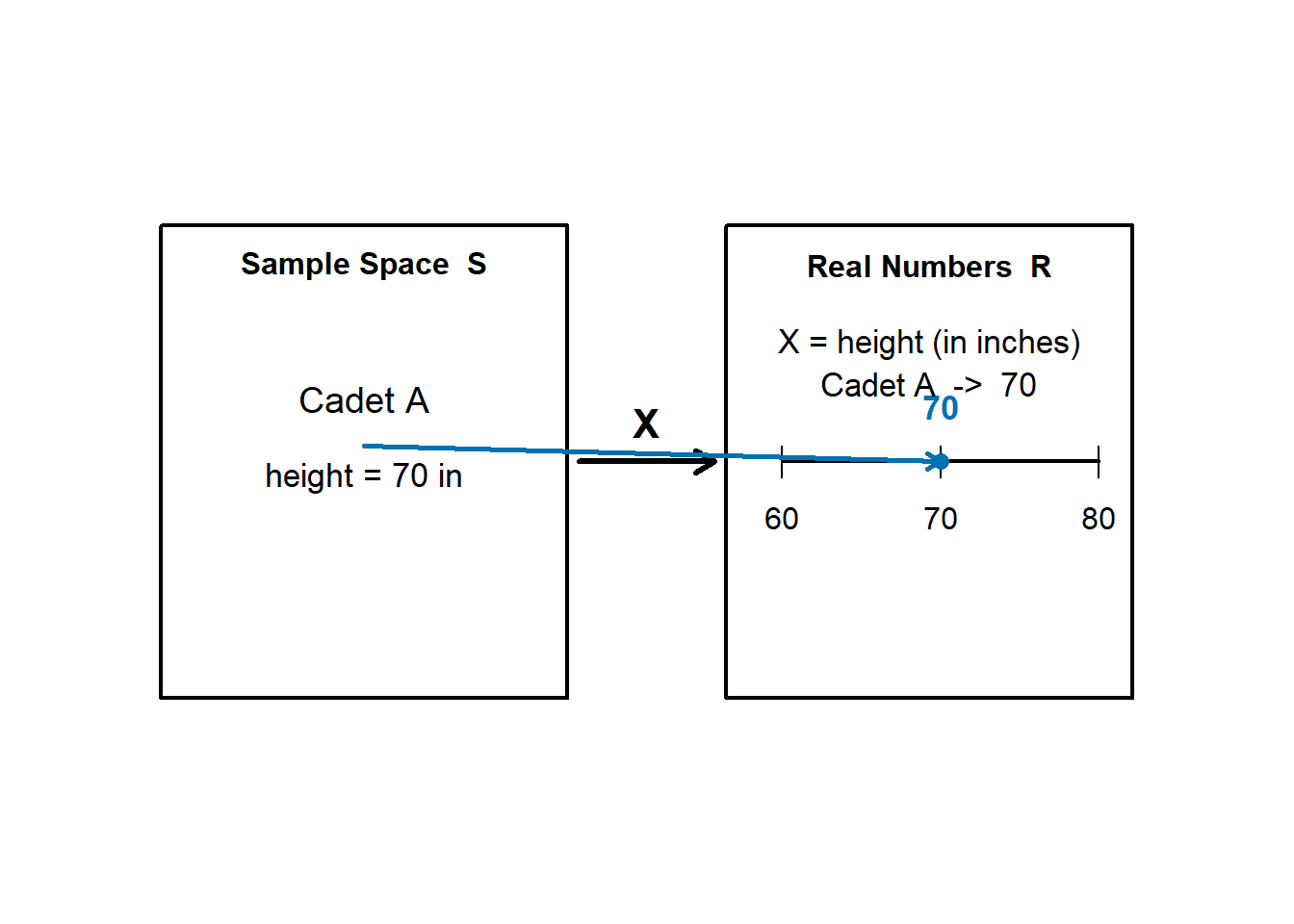
Definition: Random Variable

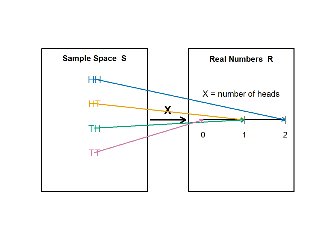
A random variable is a function that assigns a numerical value to each outcome in a sample space.

\[ X: S \rightarrow \mathbb{R} \]

We use capital letters (\(X\), \(Y\), \(Z\)) for random variables and lowercase letters (\(x\), \(y\), \(z\)) for their specific values.

A random variable is simply a rule for turning outcomes into numbers.

Example 1

Select a cadet at random and let \(X = \text{height (in inches) of the selected cadet}.\)

If the cadet is 70 inches tall, then

\[ 70 \rightarrow 70. \]

Example 2

Toss two coins with outcomes \(HH, HT, TH, TT\). Define \(X = \text{number of heads}.\)

Then

\(TT \rightarrow 0\)
\(TH \rightarrow 1\)
\(HT \rightarrow 1\)
\(HH \rightarrow 2\)

In this case, the random variable explicitly converts symbolic outcomes into numbers.

Discrete vs. Continuous Random Variables

Random variables come in two types:

Types of Random Variables

Discrete Random Variable:

Takes on a finite or countably infinite number of distinct values
Examples: Number of cadets absent, number of hits on target, count of defective items

Continuous Random Variable:

Takes on any value in an interval (uncountably infinite)
Examples: Time to complete a task, weight, distance, temperature

Today’s Focus

Today we focus exclusively on discrete random variables.

We’ll cover continuous random variables in Lesson 12.

Our Running Example

Throughout this lesson, we’ll use one example to build everything:

Example: Coin Flips

A cadet flips a fair coin 3 times.

Let \(X\) = number of heads (out of 3 flips).

What values can \(X\) take? \(X \in \{0, 1, 2, 3\}\)

We’ll use this example to teach the rest of the material for today.

Probability Mass Function (PMF)

Mathematical Definition

Definition: Probability Mass Function

The probability mass function (PMF) of a discrete random variable \(X\) is:

\[p(x) = P(X = x)\]

which gives the probability that \(X\) takes the value \(x\).

Properties:

\(p(x) \geq 0\) for all \(x\)
\(\sum_{\text{all } x} p(x) = 1\)

PMF for Our Coin Flip Example

How did we build this PMF?

Or as a formula: \(p(x) = \frac{\binom{3}{x}}{2^3}, \quad x \in \{0, 1, 2, 3\}\)

Setup: 3 coin flips, each equally likely to be H or T.

Total outcomes (ordered, with replacement): \(n^k = 2^3 = 8\) equally likely outcomes: \(\{HHH, HHT, HTH, HTT, THH, THT, TTH, TTT\}\)

Since all outcomes are equally likely, we use:

\[P(X = x) = \frac{\text{number of outcomes with } x \text{ heads}}{\text{total outcomes}} = \frac{\binom{3}{x}}{n^k} = \frac{\binom{3}{x}}{2^3}\]

Numerator: Unordered without replacement → \(\binom{3}{x}\) (choosing which flips are heads)
Denominator: Ordered with replacement → \(n^k = 2^3 = 8\) (each of 3 flips has 2 options)

Calculations:

\(P(X = 0) = \frac{\binom{3}{0}}{8} = \frac{1}{8}\) (just TTT)
\(P(X = 1) = \frac{\binom{3}{1}}{8} = \frac{3}{8}\) (HTT, THT, TTH)
\(P(X = 2) = \frac{\binom{3}{2}}{8} = \frac{3}{8}\) (HHT, HTH, THH)
\(P(X = 3) = \frac{\binom{3}{3}}{8} = \frac{1}{8}\) (just HHH)

Verify: All \(p(x) \geq 0\) ✓ and \(\sum p(x) = \frac{1+3+3+1}{8} = 1\) ✓

This uses counting! The numerator counts favorable outcomes, the denominator is the total number of equally likely outcomes.

Tabular

\(x\)	0	1	2	3
\(p(x)\)	\(\frac{1}{8}\)	\(\frac{3}{8}\)	\(\frac{3}{8}\)	\(\frac{1}{8}\)

PMF: Graphical Form

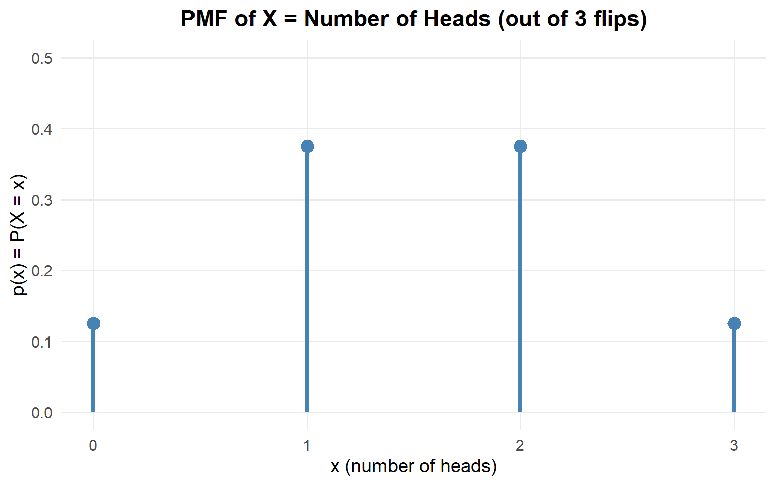
Note: For discrete RVs, we use spikes (not bars) to emphasize that probability exists only at specific points.

Formula

\[ p(X = x) = \begin{cases} \frac{1}{8} & x = 0 \\[6pt] \frac{3}{8} & x = 1 \\[6pt] \frac{3}{8} & x = 2 \\[6pt] \frac{1}{8} & x = 3 \\[6pt] 0 & \text{otherwise} \end{cases} \]

Probability Questions: Using the PMF

Now let’s use our PMF to answer some questions:

Q1: What is the probability of getting 2 or fewer heads?

\[ \begin{aligned} P(X \leq 2) &= P(X = 0) + P(X = 1) + P(X = 2) \\[6pt] &= \frac{1}{8} + \frac{3}{8} + \frac{3}{8} \\[6pt] &= \frac{7}{8} \end{aligned} \]

Q2: What is the probability of getting fewer than 2 heads?

\[ \begin{aligned} P(X < 2) &= P(X = 0) + P(X = 1) \\[6pt] &= \frac{1}{8} + \frac{3}{8} \\[6pt] &= \frac{1}{2} \end{aligned} \]

Q3: What is the probability of getting exactly 2 heads?

\[P(X = 2) = \frac{3}{8}\]

Q4: What is the probability of getting more than 2 heads?

\[P(X > 2) = P(X = 3) = \frac{1}{8}\]

Q5: What is the probability of getting 2 or more heads?

\[ \begin{aligned} P(X \geq 2) &= P(X = 2) + P(X = 3) \\[6pt] &= \frac{3}{8} + \frac{1}{8} \\[6pt] &= \frac{1}{2} \end{aligned} \]

Q6: What is the probability of getting between 1 and 3 heads?

\[ \begin{aligned} P(1 < X < 3) &= P(X = 2) \\[6pt] &= \frac{3}{8} \end{aligned} \]

Cumulative Distribution Function (CDF)

Mathematical Definition

Definition: Cumulative Distribution Function

The cumulative distribution function (CDF) of a random variable \(X\) is:

\[F(x) = P(X \leq x)\]

For a discrete RV, this is computed by summing the PMF:

\[F(x) = \sum_{y \leq x} p(y)\]

Key idea: The CDF accumulates (adds up) probabilities from the smallest value up to \(x\).

Going from PMF to CDF

To build the CDF from the PMF, we accumulate probabilities:

\[F(x) = \sum_{y \leq x} p(y)\]

For our example:

\[ p(X = x) = \begin{cases} \frac{1}{8} & x = 0 \\[6pt] \frac{3}{8} & x = 1 \\[6pt] \frac{3}{8} & x = 2 \\[6pt] \frac{1}{8} & x = 3 \\[6pt] 0 & \text{otherwise} \end{cases} \]

\(F(0) = P(X \leq 0) = p(0) = \frac{1}{8}\)
\(F(1) = P(X \leq 1) = p(0) + p(1) = \frac{1}{8} + \frac{3}{8} = \frac{4}{8} = \frac{1}{2}\)
\(F(2) = P(X \leq 2) = p(0) + p(1) + p(2) = \frac{1}{2} + \frac{3}{8} = \frac{7}{8}\)
\(F(3) = P(X \leq 3) = p(0) + p(1) + p(2) + p(3) = \frac{7}{8} + \frac{1}{8} = 1\)

CDF: Tabular Form

\(x\)	0	1	2	3
\(p(x)\)	\(\frac{1}{8}\)	\(\frac{3}{8}\)	\(\frac{3}{8}\)	\(\frac{1}{8}\)
\(F(x)\)	\(\frac{1}{8}\)	\(\frac{1}{2}\)	\(\frac{7}{8}\)	\(1\)

CDF: Graphical Form

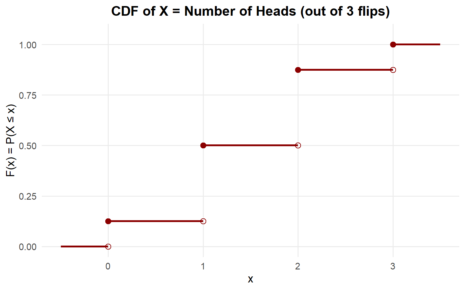
Note: The CDF of a discrete RV is a step function — it jumps at each possible value of \(X\).

CDF: Formula

\[ F(x) = \begin{cases} 0 & x < 0 \\[6pt] \frac{1}{8} & 0 \leq x < 1 \\[6pt] \frac{1}{2} & 1 \leq x < 2 \\[6pt] \frac{7}{8} & 2 \leq x < 3 \\[6pt] 1 & x \geq 3 \end{cases} \]

Probability Questions: Using the CDF

The CDF is useful for computing probabilities over ranges:

Q1: What is the probability of getting 2 or fewer heads?

\[ \begin{aligned} P(X \leq 2) &= F(2) \\[6pt] &= \frac{7}{8} \end{aligned} \]

Q2: What is the probability of getting fewer than 2 heads?

\[ \begin{aligned} P(X < 2) &= P(X \leq 1) \\[6pt] &= F(1) \\[6pt] &= \frac{1}{2} \end{aligned} \]

Q3: What is the probability of getting exactly 2 heads?

\[ \begin{aligned} P(X = 2) &= F(2) - F(1) \\[6pt] &= \frac{7}{8} - \frac{1}{2} \\[6pt] &= \frac{3}{8} \end{aligned} \]

Q4: What is the probability of getting more than 2 heads?

\[ \begin{aligned} P(X > 2) &= 1 - P(X \leq 2) \\[6pt] &= 1 - F(2) \\[6pt] &= 1 - \frac{7}{8} \\[6pt] &= \frac{1}{8} \end{aligned} \]

Q5: What is the probability of getting 2 or more heads?

\[ \begin{aligned} P(X \geq 2) &= 1 - P(X < 2) \\[6pt] &= 1 - P(X \leq 1) \\[6pt] &= 1 - F(1) \\[6pt] &= 1 - \frac{1}{2} \\[6pt] &= \frac{1}{2} \end{aligned} \]

Q6: What is the probability of getting between 1 and 3 heads?

\[ \begin{aligned} P(1 < X < 3) &= F(2) - F(1) \\[6pt] &= \frac{7}{8} - \frac{1}{2} \\[6pt] &= \frac{3}{8} \end{aligned} \]

Expected Value

What if we wanted to know the ‘expected’ number of heads in our coin flip example?

Mathematical Definition

Definition: Expected Value

The expected value (or mean) of a discrete random variable \(X\) is:

\[E(X) = \mu = \sum_{\text{all } x} x \cdot p(x)\]

Interpretation: The expected value is the long-run average — if you repeated the experiment many times, the average value of \(X\) would approach \(E(X)\).

Important Note

The expected value is NOT necessarily a value that \(X\) can actually take!

Expected Value: Our Example

\[E(X) = \sum_{x=0}^{3} x \cdot p(x)\]

\[= 0 \cdot \frac{1}{8} + 1 \cdot \frac{3}{8} + 2 \cdot \frac{3}{8} + 3 \cdot \frac{1}{8}\]

\[= 0 + \frac{3}{8} + \frac{6}{8} + \frac{3}{8} = \frac{12}{8} = 1.5\]

Interpretation: On average, you will get 1.5 heads out of 3 flips. Over many repetitions of this experiment, the average number of heads will approach 1.5.

Note: 1.5 is not a possible value of \(X\) (you can’t flip 1.5 heads), but it’s still a meaningful measure of center.

Variance and Standard Deviation

What if we wanted to know how much the number of heads varies between experiments from the expected value in our coin flip example?

Mathematical Definition

Definition: Variance

The variance of a discrete random variable \(X\) is:

\[Var(X) = \sigma^2 = E[(X - \mu)^2] = \sum_{\text{all } x} (x - \mu)^2 \cdot p(x)\]

Shortcut formula: \[Var(X) = E(X^2) - [E(X)]^2\]

Definition: Standard Deviation

The standard deviation is:

\[SD(X) = \sigma = \sqrt{Var(X)}\]

Interpretation: Variance and SD measure how spread out the distribution is around the mean.

Variance: Our Example

Method 1: Using the Definition

\[Var(X) = \sum_{\text{all } x} (x - \mu)^2 \cdot p(x)\]

\(x\)	0	1	2	3
\(p(x)\)	\(\frac{1}{8}\)	\(\frac{3}{8}\)	\(\frac{3}{8}\)	\(\frac{1}{8}\)

With \(\mu = 1.5\):

\[ \begin{aligned} Var(X) &= (0 - 1.5)^2 \cdot \frac{1}{8} + (1 - 1.5)^2 \cdot \frac{3}{8} + (2 - 1.5)^2 \cdot \frac{3}{8} + (3 - 1.5)^2 \cdot \frac{1}{8} \\[6pt] &= (2.25) \cdot \frac{1}{8} + (0.25) \cdot \frac{3}{8} + (0.25) \cdot \frac{3}{8} + (2.25) \cdot \frac{1}{8} \\[6pt] &= \frac{2.25}{8} + \frac{0.75}{8} + \frac{0.75}{8} + \frac{2.25}{8} \\[6pt] &= \frac{6}{8} = 0.75 \end{aligned} \]

Method 2: Using the Shortcut Formula

\[Var(X) = E(X^2) - [E(X)]^2\]

Step 1: Find \(E(X^2)\)

\[ \begin{aligned} E(X^2) &= \sum_{x=0}^{3} x^2 \cdot p(x) \\[6pt] &= 0^2 \cdot \frac{1}{8} + 1^2 \cdot \frac{3}{8} + 2^2 \cdot \frac{3}{8} + 3^2 \cdot \frac{1}{8} \\[6pt] &= 0 + \frac{3}{8} + \frac{12}{8} + \frac{9}{8} = \frac{24}{8} = 3 \end{aligned} \]

Step 2: Apply the shortcut formula

\[Var(X) = E(X^2) - [E(X)]^2 = 3 - (1.5)^2 = 3 - 2.25 = 0.75\]

Standard Deviation

\[SD(X) = \sqrt{Var(X)} = \sqrt{0.75} \approx 0.866\]

Interpretation: The number of heads typically varies by about 0.87 from the average of 1.5.

Summary: Our Running Example

Complete Analysis: 3 Fair Coin Flips

PMF:

\[ p(x) = \begin{cases} \frac{1}{8} & x = 0 \\[6pt] \frac{3}{8} & x = 1 \\[6pt] \frac{3}{8} & x = 2 \\[6pt] \frac{1}{8} & x = 3 \\[6pt] 0 & \text{otherwise} \end{cases} \]

CDF:

\[ F(x) = \begin{cases} 0 & x < 0 \\[6pt] \frac{1}{8} & 0 \leq x < 1 \\[6pt] \frac{1}{2} & 1 \leq x < 2 \\[6pt] \frac{7}{8} & 2 \leq x < 3 \\[6pt] 1 & x \geq 3 \end{cases} \]

Summary Statistics:

\(E(X) = 1.5\) heads
\(Var(X) = 0.75\)
\(SD(X) \approx 0.866\) heads

Board Problem: Rolling a Fair Die

A cadet rolls a fair six-sided die. Let \(X\) = the number showing on the top face.

Part A: Build the PMF

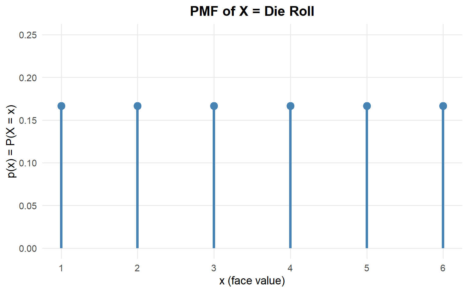
A1: What values can X take?

\(X \in \{1, 2, 3, 4, 5, 6\}\)

A2: Find the PMF in tabular form

\(x\)	1	2	3	4	5	6
\(p(x)\)	\(\frac{1}{6}\)	\(\frac{1}{6}\)	\(\frac{1}{6}\)	\(\frac{1}{6}\)	\(\frac{1}{6}\)	\(\frac{1}{6}\)

A3: Write the PMF as a formula

\[ p(x) = \begin{cases} \frac{1}{6} & x \in \{1, 2, 3, 4, 5, 6\} \\[6pt] 0 & \text{otherwise} \end{cases} \]

A4: Sketch the PMF

Part B: Build the CDF

B1: Find the CDF in tabular form

\(x\)	1	2	3	4	5	6
\(F(x)\)	\(\frac{1}{6}\)	\(\frac{2}{6}\)	\(\frac{3}{6}\)	\(\frac{4}{6}\)	\(\frac{5}{6}\)	\(1\)

B2: Write the CDF as a formula

\[ F(x) = \begin{cases} 0 & x < 1 \\[6pt] \frac{1}{6} & 1 \leq x < 2 \\[6pt] \frac{2}{6} & 2 \leq x < 3 \\[6pt] \frac{3}{6} & 3 \leq x < 4 \\[6pt] \frac{4}{6} & 4 \leq x < 5 \\[6pt] \frac{5}{6} & 5 \leq x < 6 \\[6pt] 1 & x \geq 6 \end{cases} \]

B3: Sketch the CDF

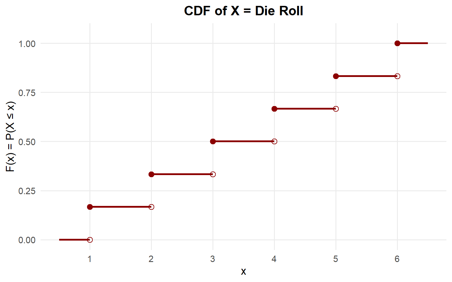
Part C: Probability Questions Using the PMF

C1: What is the probability of rolling 4 or fewer?

\[ \begin{aligned} P(X \leq 4) &= P(X = 1) + P(X = 2) + P(X = 3) + P(X = 4) \\[6pt] &= \frac{1}{6} + \frac{1}{6} + \frac{1}{6} + \frac{1}{6} \\[6pt] &= \frac{4}{6} = \frac{2}{3} \end{aligned} \]

C2: What is the probability of rolling fewer than 4?

\[ \begin{aligned} P(X < 4) &= P(X = 1) + P(X = 2) + P(X = 3) \\[6pt] &= \frac{1}{6} + \frac{1}{6} + \frac{1}{6} \\[6pt] &= \frac{3}{6} = \frac{1}{2} \end{aligned} \]

C3: What is the probability of rolling exactly 4?

\[P(X = 4) = \frac{1}{6}\]

C4: What is the probability of rolling more than 4?

\[ \begin{aligned} P(X > 4) &= P(X = 5) + P(X = 6) \\[6pt] &= \frac{1}{6} + \frac{1}{6} \\[6pt] &= \frac{2}{6} = \frac{1}{3} \end{aligned} \]

C5: What is the probability of rolling 4 or more?

\[ \begin{aligned} P(X \geq 4) &= P(X = 4) + P(X = 5) + P(X = 6) \\[6pt] &= \frac{1}{6} + \frac{1}{6} + \frac{1}{6} \\[6pt] &= \frac{3}{6} = \frac{1}{2} \end{aligned} \]

C6: What is the probability of rolling between 2 and 5?

\[ \begin{aligned} P(2 \leq X \leq 5) &= P(X = 2) + P(X = 3) + P(X = 4) + P(X = 5) \\[6pt] &= \frac{1}{6} + \frac{1}{6} + \frac{1}{6} + \frac{1}{6} \\[6pt] &= \frac{4}{6} = \frac{2}{3} \end{aligned} \]

Part D: Probability Questions Using the CDF

D1: What is the probability of rolling 4 or fewer?

\[ \begin{aligned} P(X \leq 4) &= F(4) \\[6pt] &= \frac{4}{6} = \frac{2}{3} \end{aligned} \]

D2: What is the probability of rolling fewer than 4?

\[ \begin{aligned} P(X < 4) &= P(X \leq 3) \\[6pt] &= F(3) \\[6pt] &= \frac{3}{6} = \frac{1}{2} \end{aligned} \]

D3: What is the probability of rolling exactly 4?

\[ \begin{aligned} P(X = 4) &= F(4) - F(3) \\[6pt] &= \frac{4}{6} - \frac{3}{6} \\[6pt] &= \frac{1}{6} \end{aligned} \]

D4: What is the probability of rolling more than 4?

\[ \begin{aligned} P(X > 4) &= 1 - P(X \leq 4) \\[6pt] &= 1 - F(4) \\[6pt] &= 1 - \frac{4}{6} \\[6pt] &= \frac{2}{6} = \frac{1}{3} \end{aligned} \]

D5: What is the probability of rolling 4 or more?

\[ \begin{aligned} P(X \geq 4) &= 1 - P(X < 4) \\[6pt] &= 1 - P(X \leq 3) \\[6pt] &= 1 - F(3) \\[6pt] &= 1 - \frac{3}{6} \\[6pt] &= \frac{1}{2} \end{aligned} \]

D6: What is the probability of rolling between 2 and 5?

\[ \begin{aligned} P(2 \leq X \leq 5) &= F(5) - F(1) \\[6pt] &= \frac{5}{6} - \frac{1}{6} \\[6pt] &= \frac{4}{6} = \frac{2}{3} \end{aligned} \]

Part E: Expected Value

E1: Calculate E(X)

\[ \begin{aligned} E(X) &= \sum_{x=1}^{6} x \cdot p(x) \\[6pt] &= 1 \cdot \frac{1}{6} + 2 \cdot \frac{1}{6} + 3 \cdot \frac{1}{6} + 4 \cdot \frac{1}{6} + 5 \cdot \frac{1}{6} + 6 \cdot \frac{1}{6} \\[6pt] &= \frac{1 + 2 + 3 + 4 + 5 + 6}{6} \\[6pt] &= \frac{21}{6} = 3.5 \end{aligned} \]

Interpretation: On average, the die will show 3.5 over many rolls.

Part F: Variance and Standard Deviation

F1: Calculate Var(X) using the shortcut formula

Step 1: Find \(E(X^2)\)

\[ \begin{aligned} E(X^2) &= \sum_{x=1}^{6} x^2 \cdot p(x) \\[6pt] &= 1^2 \cdot \frac{1}{6} + 2^2 \cdot \frac{1}{6} + 3^2 \cdot \frac{1}{6} + 4^2 \cdot \frac{1}{6} + 5^2 \cdot \frac{1}{6} + 6^2 \cdot \frac{1}{6} \\[6pt] &= \frac{1 + 4 + 9 + 16 + 25 + 36}{6} \\[6pt] &= \frac{91}{6} \approx 15.167 \end{aligned} \]

Step 2: Apply the shortcut formula

\[ \begin{aligned} Var(X) &= E(X^2) - [E(X)]^2 \\[6pt] &= \frac{91}{6} - (3.5)^2 \\[6pt] &= \frac{91}{6} - \frac{73.5}{6} \\[6pt] &= \frac{17.5}{6} \approx 2.917 \end{aligned} \]

F2: Calculate SD(X)

\[SD(X) = \sqrt{Var(X)} = \sqrt{\frac{17.5}{6}} \approx 1.708\]

Interpretation: The die roll typically varies by about 1.7 from the average of 3.5.

Before You Leave

Today

A random variable maps outcomes to numbers
Discrete RVs take finite/countable values
PMF: \(p(x) = P(X = x)\) with properties \(p(x) \geq 0\) and \(\sum p(x) = 1\)
CDF: \(F(x) = P(X \leq x) = \sum_{y \leq x} p(y)\)
Expected Value: \(E(X) = \sum x \cdot p(x)\) — the long-run average
Variance: \(Var(X) = E(X^2) - [E(X)]^2\) — measures spread

Any questions?

Next Lesson

Lesson 10: Binomial Distribution

Verify binomial conditions for counts of successes
Compute binomial PMF/CDF values
Interpret binomial mean and variance

Upcoming Graded Events

WebAssign 3.1, 3.2, 3.3 - Due before Lesson 10
Exploratory Data Analysis - Due Lesson 9
WPR I - Lesson 16